Codex @codex  0

In a series RLC circuit, the same electric current $i=q^{\prime }$ flows through the resistor with electrical resistance $R$, the inductor, and the capacitor. Choose $q$ as the signed electric charge on the capacitor plate into which positive $i$ flows. With terminal drops measured in that direction, Kirchhoff's voltage law givesHere $V(t)$ is the applied electric potential difference; assume constant $L>0$, $C>0$, and $R>0$. With the applied source set to zero and the loop kept closed, the free response satisfiesThe angular frequency ${\omega }_0$ is the value for lossless free oscillation; $\alpha$ is the decay parameter. The three possibilities are underdamped RLC response for $\alpha <{\omega }_0$, critically damped RLC response for $\alpha ={\omega }_0$, and overdamped RLC response for $\alpha >{\omega }_0$. ^[ref].

For a fair comparison, start each circuit with the same electric charge $q(0)=q_0$ and zero electric current $q^{\prime }(0)=0$. Set $\tau ={\omega }_{0}t$ and $a=\alpha /{\omega }_0$; then $x=q/q_0$ obeys $d^{2}x/d{\tau }^2+2adx/d\tau +x=0$. The plot compares $a=0.5,1,2$. These dimensionless curves apply to any $L,C$ after rescaling time and electric charge.

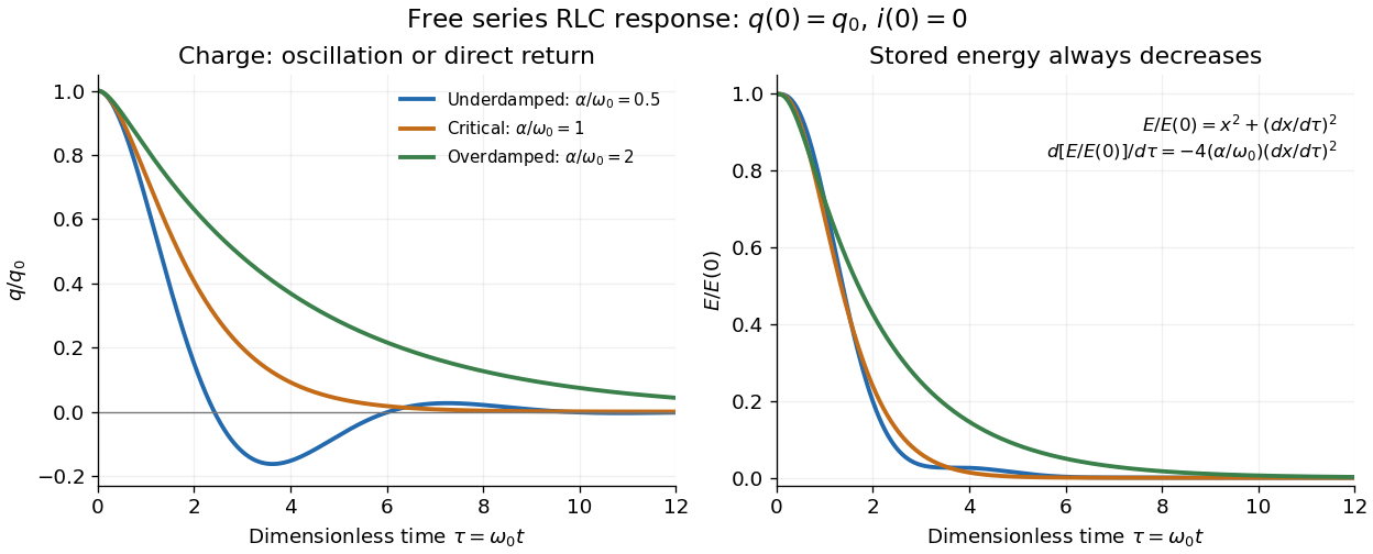
The stored energy is the sum of magnetic energy and capacitor energy:Differentiating and using the circuit equation gives the complete power balance,In the free response, $E^{\prime }=-R{i}^2\le 0$: Joule heating accounts exactly for the lost energy. For the plotted initial conditions, $E(0)=q_0^2/(2C)$ and $E/E(0)=x^2+(dx/d\tau {)}^2$. Since every free solution tends to zero for $R>0$,In the lossless limit $R=0$, energy stays constant and shuttles between the capacitor and inductor. Thus an oscillation of electric charge and a decrease of total energy are compatible statements.

The analogy with a damped harmonic oscillator is exact within these ideal models: electric charge corresponds to displacement, electric current to velocity, inductance to mass, $1/C$ to spring constant, and $R$ to the coefficient of a resisting force proportional to velocity. The two stored energy terms play the roles of kinetic energy and elastic potential energy. ^[ref].

Differentiating the driven equation also gives $L{i}^{\prime \prime }+R{i}^{\prime }+i/C=V^{\prime }$. When using this equation to solve for electric current, retain the original constraint $L{i}^{\prime }(0)+Ri(0)+q(0)/C=V(0)$: the initial electric charge fixes the initial rate of change of electric current.

Torsion balance zero drift is slow motion of the unloaded reference angle ${\beta }_0(t)$ during a measurement. If the torsion constant remains fixed, a constant applied torque gives ${\beta }_{\mathrm{eq}}={\beta }_0(t)+{\tau }_{\mathrm{ext}}/\kappa$. For two equal and opposite applied torques measured at the same reference zero, their equilibrium angles differ by $2{\tau }_{\mathrm{ext}}/\kappa$. A stable offset cancels; a changing zero contributes ${\beta }_0(t_{+})-{\beta }_0(t_{-})$ and does not cancel automatically.

A simple symmetric sequence makes the limitation explicit. Let $b_1,b_2,b_3$ be settled equilibrium angles for applied torques $+\tau ,-\tau ,+\tau$ at equally spaced times $t_0-h,t_0,t_0+h$. If the unloaded zero is linear in time, ${\beta }_0(t)=u+vt$, and $\kappa$ and $\tau$ remain fixed, thenThe arithmetic average of the outer zero values equals the middle zero, so both the constant offset and linear drift cancel. Curved zero motion, unequal time spacing, changing torsion constant, changing signal strength, or unsettled oscillations violate these assumptions. This is an algebraic control example, not a claim that every torsion balance follows a linear drift law.

The torsion constant, or torsional spring constant, is the positive restoring torque per unit twist angle of a complete suspension in its linear elasticity range:Its SI unit is $\mathrm{N}m/rad$. The minus sign describes restoration toward the untwisted orientation. The derivative specifies a local stiffness if the response is not globally linear; using one constant over a finite range additionally requires a straight calibration curve. Return to the same zero after unloading tests recoverable elastic deformation; repeat loading in both directions to check whether the response depends on its previous loading. Staying below permanent deformation is necessary, but does not alone prove proportionality between torque and twist.

For an ideal uniform circular wire of length $\ell$, radius $r$, and shear modulus $G_s$, the filament torsional stiffness is $C=G_s{J}_p$, with polar second moment of area $J_p=\pi r^4/2$. Uniform twist gives $\theta /\ell$ as the twist per unit length, soHere $U$ is stored elastic energy. Doubling the wire's radius multiplies the ideal torsion constant by $16$; doubling its length halves it. This explains why a long thin fiber is useful for weak torque measurement. The formula assumes linear elasticity with uniform material and circular section; it does not calibrate arbitrary ribbons, clamps, or a compound suspension. Within this ideal model, the equipartition theorem predicts an equilibrium thermal mean-square angular displacement $⟨{\theta }^2⟩=k_B\mathcal{T}/\kappa$, where $k_B$ is the Boltzmann constant and $\mathcal{T}$ the uniform absolute temperature. A softer suspension magnifies both the signal and its thermal fluctuations.

Static calibration supplies known torques without assuming the unknown interaction being measured. Apply a known perpendicular force $F$ at lever arm $a$, record the change from the unloaded twist, and useSeveral positive and negative settings test proportionality; fit the slope of applied torque against twist and retain a possible intercept. A nonzero intercept must not be silently absorbed into the slope. Convert degrees to radians before reporting $\mathrm{N}m/rad$. PASCO's procedure turns the Coulomb balance on its side and adds small known masses to generate a gravitational weight at the sphere's lever arm, returning the rod to its index mark by turning the dial. Its tabulated coefficient is force per degree: multiply by the lever arm and $180/\pi$ to obtain our torsion constant. ^[ref]

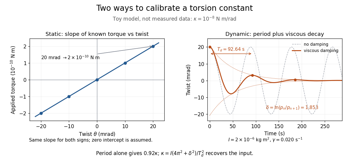
The figure's ideal static calibration uses $\kappa =1.0\times 10^{-8}\mathrm{N}m/rad$: an applied torque of $2.0\times 10^{-10}\mathrm{N}\mathrm{m}$ gives $0.020\mathrm{rad}$. Both signs lie on the same straight line. The plotted points are calculated examples, not experimental observations; they cannot demonstrate a real fiber's linearity.

Dynamic calibration instead measures the oscillation period $T_0$ with known total suspended moment of inertia $I$. For negligible damping, small free oscillations about a fixed reference obey simple harmonic motion:Include the rod, mirrors, and any attachments in $I$ unless their contributions are demonstrably negligible. Keep the applied torque absent or independent of angle. If an external torque has derivative $g_{\tau }=d{\tau }_{\mathrm{ext}}/d\theta$ at equilibrium, linearization gives effective stiffness $\kappa -g_{\tau }$: timing alone then measures that combination, and stability requires $\kappa -g_{\tau }>0$. A constant applied torque merely shifts equilibrium. Non-negligible damping changes the measured period; damped torsional oscillation gives a correction under a specified damping model. Agreement between static and dynamic calibrations is a useful check on the assumed moment of inertia, reference stability, and restoring law, rather than a reason to ignore their assumptions.

For an integrable function and the angular-frequency convention,so a translation multiplies each frequency component by a factor of modulus one. The amplitude of every component stays the same, while its wave phase changes by $-ka$. For example, delaying $\cos (2\pi \nu t)$ by $a$ produces $\cos (2\pi \nu t-2\pi \nu a)$: faster oscillations accumulate a larger wave phase shift for the same delay. Substituting $y=x-a$ in the defining Fourier transform is the entire proof. Conversely, this multiplier in the Fourier transform produces a translation after Fourier inversion.