Past exam of the approximation theory and finite element methods course of the University of Oxford / 2007 / A (Approximation Theory)

Assume $A$ is nonempty, as is necessary for an approximating point to exist. The reverse triangle inequality givesThus the distance from the fixed point $u$ is a continuous, indeed Lipschitz continuous, real-valued function on $A$. A continuous function on a nonempty compact set attains its minimum, so some $p\in A$ satisfiesIf empty compact sets are allowed, the printed statement needs this nonemptiness qualification.

The vector subspace contains zero, whose approximation error is $\Vert u\Vert$. For any $q$ with $\Vert q\Vert >2\Vert u\Vert$, the triangle inequality gives $\Vert u-q\Vert \ge \Vert q\Vert -\Vert u\Vert >\Vert u\Vert$, so such points cannot improve on zero.

Restrict to $K=\{q\in A:\Vert q\Vert \le 2\Vert u\Vert +1\}$. This is nonempty, closed and bounded in a finite-dimensional normed space, hence compact. The continuous function $q\mapsto \Vert u-q\Vert$ attains a minimum on $K$ by part (a). Outside $K$ its value exceeds the error at zero, so that minimizer is best on all of $A$:Completeness of the ambient space is unnecessary; compactness is used only in the finite-dimensional vector subspace.

The geometry of a strictly convex normed space proves uniqueness whenever a best approximation exists. If distinct $p_1,p_2$ both have best error $E>0$, then their two residuals have norm $E$. The defining midpoint inequality givescontradicting best approximation because the midpoint lies in $A$. If $E=0$, both approximants equal $u$.

The printed existence assertion is false for an arbitrary vector subspace. For a concrete counterexample take $B={\ell }^2$ with its strictly convex Hilbert norm, let $A=c_{00}$ be its finite-support sequences, and take $u=(2^{-j}{)}_{j\ge 1}$. Truncations in $A$ tend to $u$, so the best-error infimum is zero, but $u\notin A$ and that infimum is not attained. If the finite-dimensional assumption of part (b) is retained, it supplies existence and the argument above supplies uniqueness.

For the estimate, suppose $Y$ is a projection operator onto $A$, as needed for a finite operator norm. Since $Yp=p$,The triangle inequality and operator norm giveThe estimate actually holds without attainment: apply it with any $q\in A$ instead of $p$ and take the infimum. Its proof applies in every normed space. This is strict convexity separates uniqueness from existence in best approximation.

Write the Fourier coefficients as $c_k=(2\pi {)}^{-1}{\int }_{-\pi }^{\pi }u(t)e^{-ikt}dt$. The partial sum through frequencies $-n,\dots ,n$ is therefore a convolution withThe last expression follows by summing a finite geometric series, with its removable value $2n+1$ at zero. Periodicity and the evenness of $D_n$ giveThis also proves linearity and that the image lies in $F_n$. We use the continuous periodic function space, consistent with the premise and the displayed maximum norm.

The convolution formula gives the upper boundTo prove sharpness within continuous functions, takeIt is continuous and periodic, with norm at most one. At $x=0$, dominated convergence gives $(S_n{u}_{ϵ})(0)\to (2\pi {)}^{-1}\int |D_n|$. Hence that upper bound is the actual operator norm. Evenness yieldsThe approximating continuous signs avoid assuming that the discontinuous sign of the kernel belongs to the domain space.

Use the usual approximation-space convention $P_n=\{p:\mathrm{deg}p\le n\}$. The source's phrase “degree $n$” must include lower degrees for its later space and interpolation statements; the consequence of a literal exact-degree reading is addressed in part (d).

Order the alternating points as $x_0<\cdots <x_{n+1}$. If $q$ had strictly smaller error than $E_n$, the valueswould have the alternating signs of $(u-p)(x_j)$: the second term has magnitude strictly less than $E_n$. The intermediate value theorem would then give at least $n+1$ distinct zeros of $q-p$, one in each gap. A nonzero polynomial of degree at most $n$ cannot have that many zeros. Thus no such $q$ exists, provingThe remainder of the equioscillation theorem says that a best uniform approximating polynomial exists, is unique, and is characterized by this $n+2$-point alternating extreme-error condition. For positive error, alternation is necessary as well as sufficient. If $u$ itself lies in $P_n$, the unique best polynomial is $u$ with zero error.

Let $\omega (t)={\prod }_{r=0}^n(t-x_r)$. For $x$ not one of the nodes, put $c=(u(x)-p_n(x))/\omega (x)$ and defineThis function has zeros at the $n+1$ interpolation nodes and at the additional point $x$. Repeated Rolle's theorem gives a point $\eta$ between the outermost of these points such that $F^{(n+1)}(\eta )=0$. Since $p_n^{(n+1)}=0$ and ${\omega }^{(n+1)}=(n+1)!$,Substitution yieldsAt an interpolation node both sides are zero, so any $\eta \in [-1,1]$ gives the identity there. The assumed $C^{n+1}$ regularity permits all applications of Rolle's theorem.

Choose the nodes as the $n+1$ roots of the Chebyshev polynomial $T_{n+1}$. Its leading coefficient is $2^n$, so the monic nodal product is $\omega =2^{-n}{T}_{n+1}$. Since $|T_{n+1}|\le 1$ on $[-1,1]$, part (b) bounds this particular interpolant byThe best error cannot exceed the error of a particular member of $P_n$. ThereforeThe choice of Chebyshev roots controls the maximum of the nodal product, not the size of any individual interpolation coefficient.

The polynomial $T_6$ isSubtract its monic version from $x^6$:This has degree four and hence belongs to the usual space $P_5$. The error is $T_6/32$, with norm $1/32$ and alternating extrema at the seven points $\cos (j\pi /6)$, $j=0,\dots ,6$. Part (a), followed by uniqueness, provesand that this is the unique best approximation of degree at most five.

If “degree five” is taken literally to exclude degree four, no best approximation exists in that nonclosed class: $p+ϵx^5$ approaches the error $1/32$ as $ϵ\to 0$, but uniqueness in $P_5$ excludes attainment by any degree-five polynomial. This is why the standard at-most-degree convention matters here.

If $(u-p,q)=0$ for all $q\in A$, then for any $a\in A$ the difference $p-a$ lies in $A$ and Pythagorean theorem givesThus $p$ is best.

Conversely, if $p$ is best, then for every $q\in A$ the real quadratichas its minimum at $t=0$. Its linear coefficient must vanish, giving $(u-p,q)=0$. Hence best approximation is equivalent to orthogonality of the residual to the approximation space. The weight is positive almost everywhere, so this is a genuine positive-definite inner product on continuous functions.

For the weighted inner product, $(x^j,x^k)=1/(j+k+2)$. Start Gram-Schmidt process with the monomials and choose monic normalization:Its squared norm is $1/4-4/9+2/9=1/36$. Next $(x^2,1)/(1,1)=1/2$ andThereforeSubtracting these orthogonal projections gives orthogonality by construction; independent nonzero rescalings would give equivalent unnormalized orthogonal polynomials.

Write $p=a+bx$. orthogonality of the residual to $1,x$ givesThe first integral follows from $t=1-x^2$; for the second use $x=\sin \theta$, giving ${\int }_0^{\pi /2}{\sin }^2\theta {\cos }^2\theta d\theta =\pi /16$. The coefficient matrix has determinant $1/72$, so solving yieldsPart (a) proves this is the unique best weighted $L^2$ approximation. The weight $x$ is essential; using ordinary unweighted normal equations would give different coefficients.

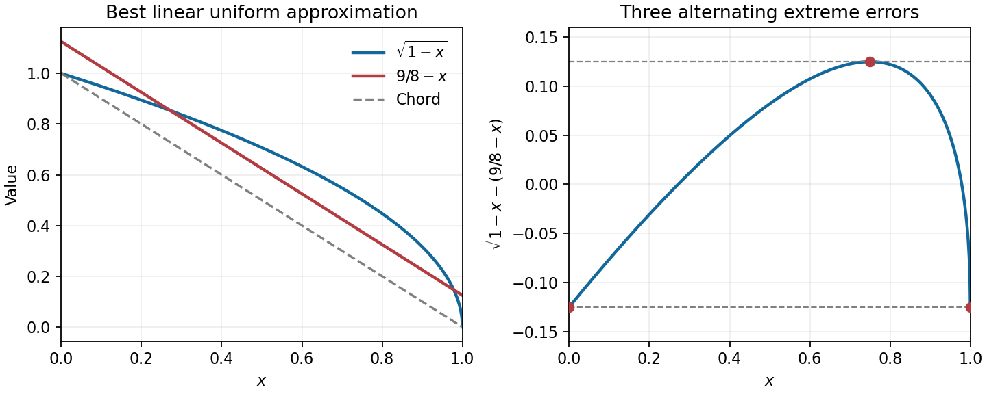
The endpoint chord is $l(x)=1-x$. Since the square-root function is concave, the gap $g(x)=\sqrt{1-x}-(1-x)$ is nonnegative. Put $t=\sqrt{1-x}$ to obtain $g=t-t^2$, whose maximum is $1/4$ at $t=1/2$, or $x=3/4$.

Shift the chord upward by half that maximum. ThenThe errors at $x=0,3/4,1$ are respectively $-1/8,+1/8,-1/8$. These are three alternating extrema, so equioscillation proves optimality and uniqueness for linear polynomials. This is minimax linear approximation of a square-root endpoint profile.

Use the Taylor expansion $\sqrt{1-x}=1-x/2-x^2/8+O(x^3)$. Expanding the rational form givesMatching through degree two yields $a_0=1$, $a_1-b_1=-1/2$, and $b_1^2-a_1{b}_1=-1/8$. The last equation becomes $b_1/2=-1/8$, soThis is the $[1/1]$ Padé approximant about zero. Its pole is at four, outside the interpolation interval; its order of matching is local and does not assert uniform minimax optimality.

Let $\beta (q)$ be the centered nondimensional cubic B-spline, even and supported on $[-2,2]$. The outer cubic must be $b(2-|q|{)}^3$ to make the function and its first two derivatives vanish at the support edge. Write its inner part as $A+B{q}^2+C|q{|}^3$. Matching the value and first two derivatives at $|q|=1$ gives $A=4b$, $B=-6b$, $C=3b$. Its nonzero knot values are then $4b,b,b$, so requiring their sum to be one fixes $b=1/6$. ThusIn particular $\beta (0)=2/3$, $\beta (\pm 1)=1/6$.

With $h=1/m$, represent the spline on $[0,1]$ as $s(x)={\sum }_{j=-1}^{m+1}{c}_j\beta (x/h-j)$. There are $m+3$ unknown coefficients. interpolation at $x_i=ih$, $0\le i\le m$, givesThe natural endpoint conditions, using ${\beta }^{\prime \prime }(0)=-2$ and ${\beta }^{\prime \prime }(\pm 1)=1$, giveThese $m+3$ equations are the required matrix system: the $m+1$ interpolation rows have coefficients $(1,4,1)$ at consecutive positions and right sides $6u(x_i)$; the two endpoint rows have $(1,-2,1)$ and zero right sides. No solution of that system is required. The scaling uses $\beta (x/h-j)$, without an extra $1/h$, because normalization is by knot values rather than by integral.