A shock wave forms when a compressive flow steepens or when gas must be decelerated or turned faster than upstream acoustic waves can communicate the change. Astrophysical examples include a supernova remnant sweeping up surrounding gas, a fast stellar wind colliding with ambient material, and supersonic accretion onto an obstacle or onto a dense gas layer. A large Mach number by itself is not sufficient: a uniform supersonic stream need not contain a shock wave.
Choose the shock frame, and denote upstream and downstream normal velocities by . Integrating the local conservation laws over a thin control volume spanning a steady normal shock wave gives equal fluxes on both sides. Mass conservation gives constant mass flux per unit area,Pressure and advected momentum together give the normal momentum flux,For a thin non-radiating layer, with negligible gravitational-potential change across it, conservation of energy gives equal fluxes . A perfect gas has specific enthalpy , soThese are the Rankine-Hugoniot conditions for a perfect gas. Dissipation inside the thin layer produces an entropy increase and selects the physical compressive branch. Efficient radiative cooling would change the energy relation and may instead lead to an isothermal shock.
Take . Let . Mass conservation gives , and normal momentum conservation givesInsert this into the energy condition from part (a):Rearranging and factoring,The root is the unshocked state. The compressive Strong-shock Rankine-Hugoniot conditions instead giveCorrespondingly, and . These relations require and negligible upstream thermal pressure.
Let denote the total flow speeds, keeping the normal components distinct from them. The original diagram measures from the initial wall direction to the shock wave itself. The outgoing velocity is turned by , so it makes angle with the shock.
Resolve each velocity tangent and normal to the oblique shock. Tangential momentum conservation, with nonzero mass flux and no tangential surface force, makes the tangential velocity continuous:The normal flow obeys the strong normal shock wave result from part (b):Divide the second relation by the first to obtainThe approximation is controlled by the upstream normal Mach number , not just by . This distinction matters on the small-angle weak branch in part (d). The angle convention is also important: formulas using the angle to the shock normal instead would interchange sine and cosine.
Rewrite the relation from part (c) asThe angle-addition identities reduce this toFor , the right side lies strictly between zero and one. There are two physically admissible strong oblique-shock angle branches:Both lie between and . They merge when , proving the maximum deflection through a strong perfect-gas shock,For small positive , the formal strong-shock-limit asymptotics areThe weak branch is normally observed for an unconfined supersonic stream turning through a modest compression corner. It has a smaller normal component of upstream velocity, hence a smaller downstream pressure increase; for small turns the downstream flow remains supersonic. The nearly normal strong branch can be selected by suitable downstream pressure conditions, so it is not mathematically forbidden.
The two limits must be ordered honestly. At finite , the weak oblique shock approaches the Mach angle as , rather than zero. The displayed weak-branch asymptotic applies when the large- limit is taken first, or in the overlapping range , where remains valid.
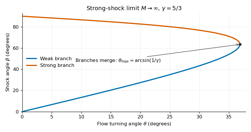
Calculated weak and strong shock-angle branches in the infinite-Mach-number limit, for a monatomic gas
. Details. 
For , , so there is no real solution for an attached straight oblique shock satisfying the assumed geometry. The shock detaches and becomes curved, with a locally strong, nearly normal portion and a subsonic region allowing the flow to adjust to the wall. The precise detached structure depends on the global geometry and downstream conditions; the attached-shock formula cannot be continued to these turns.
Let be the enclosed mass. For spherical symmetry, hydrostatic equilibrium and mass conservation giveThe isothermal equation of state therefore impliesMultiply by , differentiate and eliminate :or equivalently . This is the density equation for an isothermal sphere. Here has units and equals the squared isothermal sound speed.
A regular isothermal sphere does not reach zero density at a finite radius. The finite body discussed later must therefore be truncated by a nonzero external pressure, as in a pressure-confined isothermal sphere. A finite vacuum boundary would not be compatible with this equation of state.
Set and . Then and the equation from part (a) becomesWith , the coefficients cancel, giving the isothermal Lane-Emden equationThe regular central boundary conditions areThe first makes the central mass density equal to . The second follows from smooth spherical symmetry and the vanishing central gravitational acceleration; a preferred radial slope at the origin would be singular. Substitution of a regular power series giveswhich supplies nonsingular starting data for numerical integration. The central conditions select the regular solution, not the singular isothermal sphere.
The particle count is the enclosed mass divided by the particle mass :Integrating the isothermal Lane-Emden equation giveswhere regularity makes the lower endpoint vanish. ThusThe prefactor is a mass divided by a mass, and the remaining factor is dimensionless. In particular, at fixed the dependence on central mass density is , with . Both changes must be retained when comparing equilibria at fixed .
Along a family of equilibria at fixed temperature, and the dimensionless function are fixed. The boundary mass density changes through both and the boundary coordinate :From part (c), , where is constant at fixed temperature and . Set its logarithmic variation to zero:The isothermal Lane-Emden equation gives , so the fixed- relation isSubstitute back into the boundary-density variation:For a nontrivial variation at a finite positive radius, its vanishing gives the fixed-mass turning point of an isothermal sphere:This derivative follows a fixed-mass sequence of equilibria; it is not merely the spatial derivative of density inside one sphere. The corresponding radial variation isAt small , : the boundary density increases while the radius decreases along increasing , giving the stated negative of the stable branch. The first density turning point marks its first loss of radial stability; it need not be confused with a turning point of radius itself.
Using the supplied first critical value , the critical radius of a pressure-confined isothermal sphere isNo radius in metres can be specified without and a central mass density. Here is the isothermal sound speed, consistent with the fixed-temperature variations in part (d). At a given central mass density, equilibria truncated at lie on the first stable branch, while increasing the dimensionless outer radius beyond this first threshold gives an unstable configuration. Numerical integration gives , consistent with the paper's rounded .
For a transparent comparison with the given Jeans length, set the uniform comparison density and use the same speed of sound. ThenBoth scales express the competition between pressure support and self-gravity, with characteristic length . Their numerical closeness under this density choice does not mean that the models impose the same threshold: is a boundary radius, whereas is the wavelength of a perturbation. Comparing with would instead give a factor about . Using the sphere's mean or boundary density instead of its central density changes the coefficient again, so the reference density must always be stated.
The pressure-confined isothermal sphere gives an actual finite, centrally concentrated hydrostatic equilibrium and an explicit confining pressure, making its radial stability threshold more self-consistent for a roughly spherical isothermal cloud. The uniform Jeans instability model gives a simpler local criterion, includes perturbations at different wavelengths, and does not require constructing a spherical equilibrium. Its ideal uniform static infinite background requires the Jeans swindle or an explicitly specified treatment of background gravity. Neither model includes rotation, magnetic fields, turbulent support or a realistic temperature evolution, so neither is a universal collapse criterion.
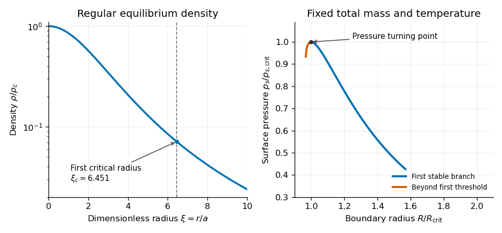
Numerically integrated isothermal-sphere density profile and the first pressure turning point along a fixed-mass sequence
. Details. 
For a steady axisymmetric flow , incompressible flow is automatic. The only material acceleration is centripetal, . The radial Euler equations therefore requireWith no viscosity there is no tangential shear stress to redistribute angular momentum. Any sufficiently regular can therefore be a steady inviscid profile, with the radial pressure adjusted by integrating this equation. This is a statement of equilibrium, not of stability: some such profiles are centrifugally unstable.
For a homogeneous Newtonian fluid with constant kinematic viscosity , assume the same steady purely azimuthal flow. In cylindrical coordinates, the azimuthal Navier-Stokes equation has no pressure forcing or convective term in this state, and becomesEquivalently, , or . Two integrations give the steady circular Couette profile,This is the basic Taylor-Couette flow between rotating cylinders. The constants depend on boundary angular velocities; for radii and prescribed angular velocities ,If the domain includes , regularity requires , leaving solid-body rotation. On an annulus a nonzero is allowed and wall torques maintain the shear.
The restriction concerns a steady profile. An arbitrary initial angular velocity does not cease to exist when viscosity is introduced; within the purely azimuthal ansatz it evolves according to until compatible boundary conditions and angular-momentum constraints determine its long-time state.
Expand the axisymmetric Euler equations about the rotating equilibrium, retaining only terms linear in and in the pressure perturbation. The symbol in this question is the kinematic pressure perturbation,The linearized centripetal term in the radial equation is , after subtracting the equilibrium term . Radial advection of the background azimuthal velocity, together with the cylindrical-coordinate term , givesThis is the azimuthal coupling in the second equation; it also expresses conservation of specific angular momentum for a radially displaced element. The axial equation is acceleration balanced by . Finally, the axisymmetric incompressible flow condition in cylindrical coordinates iswhich expands to the last supplied equation. Background azimuthal advection contributes no term because the perturbations are axisymmetric.
Use the thin-annulus approximation stated in the source, so . LetHere is the conventional Rayleigh discriminant, also the squared local radial epicyclic frequency when positive. For and , the azimuthal and axial mode equations giveThe thin-gap incompressible flow condition then gives . Substitute these into the radial equation:ThusTo put this into exactly the form printed in the paper, defineThe narrow-gap centrifugal stability equation is consequentlyThe two rigid cylinders are impermeable, so the no-penetration boundary condition givesThere is no inviscid no-slip condition on the tangential or axial components.
The sign deserves emphasis: the source's printed plus sign makes its the negative of the conventional Rayleigh discriminant. Using the conventional positive discriminant instead requires a minus sign in front of that potential term. These are equivalent conventions; replacing one without adjusting the other would falsely predict instability of solid-body rotation. The and marginal cases, excluded by these eliminations, must be treated separately or by limits.
Let be a nonzero admissible mode, multiply the equation of part (d) by its complex conjugate and integrate between the cylinders. The endpoint conditions remove the boundary term in integration by parts, giving the Rayleigh stability integral identityRearrange to obtain a real Rayleigh quotient:The denominator is strictly positive. Consequently, with the paper's convention,The weak inequality excludes exponentially growing axisymmetric modes, but permits marginal cases and possible algebraic growth when the restoring effect vanishes. Strict negativity avoids that degeneracy. Equivalently, the conventional Rayleigh discriminant is positive, or the squared specific angular momentum increases outward:This is the Rayleigh centrifugal stability criterion. In the suggested Time-independent Schrödinger equation analogy, a growing mode has ; if , its effective potential is nonnegative. The nonnegative kinetic term and that potential cannot have the required negative eigenvalue , which gives the same exclusion.
As a sign check, for solid-body rotation and . In a gap of width , the radial modes haveas expected for inertial waves. The argument establishes axisymmetric inviscid stability within the stated thin-gap model, rather than a claim about all perturbations of a viscous flow.
Articles by others on the same topic
There are currently no matching articles.