A fluid particle follows a Lagrangian trajectory, so its position satisfies rather than the velocity evaluated permanently at its initial position. Assume , and writeSet and . A Taylor expansion of the velocity about givesThus , andAt the next order,so the required second-order trajectory in a sinusoidal velocity field isBoth corrections vanish at . All retained terms have units of length. The secular contribution gives the Stokes driftalthough the Eulerian time average of the given velocity is zero. The particle samples the wave at its displaced position, producing this second-order drift. The expansion is in the dimensionless parameter , for fixed times; it ceases to be uniform when the accumulated drift changes the wave phase by order unity.
Interpret “reach” first as remaining an energetic, supersonic blast wave, rather than as the arrival of any acoustic wave. An atmospheric blast-wave range estimate must account for the thin atmosphere: the distance is much greater than its height .
For an optimistic estimate, suppose the deposited energy remains in a horizontally expanding atmospheric layer. If its representative mass density is , the swept mass is of order . Conservation of energy gives the self-similar blast wave scalingUsing ordinary atmospheric estimates and speed of sound , this givesThese are scaling estimates, not an exact shock wave solution. The strong shock wave approximation would already have failed atEquivalently, keeping the disturbance strongly supersonic out to would require substantially more than the sonic-transition energy scalewhich exceeds by about a factor of twenty. Reasonable atmospheric averages and order-unity geometrical coefficients do not reverse the comparison. Escape of energy through the top of the atmosphere makes the fully confined estimate optimistic; Earth's curvature changes its area estimate by an order-unity factor.
The strong atmospheric blast will not survive to Lansing in this model. A weakened acoustic wave can nevertheless travel there. The supplied energy and atmospheric height do not determine its detectable amplitude, detailed attenuation or damage: those require an atmospheric propagation model. Thus “no disturbance of any kind reaches Lansing” would be an unjustified stronger conclusion.
This is magnetic flux freezing in ideal magnetohydrodynamics. In addition to the supplied ideal magnetohydrodynamic induction equation, a physical magnetic field obeys Gauss's law for magnetism, .
Parameterize the material surface by two particle labels , so and . Differentiating these tangents gives the material surface element evolution lawwhere . Thus the material magnetic-flux transport theorem isExpand the curl in the ideal magnetohydrodynamic induction equation:Since is the material derivative, the first three terms cancel the corresponding terms in the surface transport formula. The remaining integrand is . ThereforeNo incompressible flow assumption is needed: the changing surface area cancels the compression term. This proof assumes smooth velocity and magnetic field and a surface carried with the fluid; the ideal magnetohydrodynamic induction equation by itself, for an arbitrary non-solenoidal vector field, would leave the final divergence term.
The buoyancy frequency, also called the Brunt–Väisälä frequency, is the angular frequency of a small vertical displacement restored by buoyancy in a stably stratified fluid. Take upward, gravitational acceleration , and a background in hydrostatic equilibrium,Displace a small gas element upward by , sufficiently slowly for its pressure to match its surroundings but without heat exchange. For this adiabatic process, is constant along the element's motion, so its mass density changes by . The surrounding mass density changes by . The element's excess mass density is consequentlyIts acceleration is . ThusFor a gas of fixed composition obeying the ideal gas law, . The adiabatic buoyancy frequency of an ideal gas is thereforewhere is the specific heat capacity at constant pressure, and is the specific gas constant. Here has units ; is an angular frequency, not a cyclic frequency. Positive gives simple harmonic motion, negative gives convective instability, and is marginal. The temperature form assumes fixed composition; the preceding density form is more general.
Write the background mass density as and its hydrostatic pressure as , whereApply an Eulerian perturbation of a fluid variable to the background fields:Thus is the Eulerian pressure perturbation, in pascals; it is not the background hydrostatic pressure.
For incompressible flow, mass conservation becomes . Linearizing about rest givesThe Euler equations are . The background pressure gradient and weight cancel. Dropping products of perturbations givesUnder , replace by in inertia but retain the background mass density gradient in the displacement-induced buoyancy. This is the Boussinesq approximation. Its linear Boussinesq equations here areThe absolute value makes explicit that the small-density-variation condition concerns magnitude, including the usual negative of stable density stratification.
Use plane wave perturbations proportional to , with amplitudes . The linear equations becomeTo eliminate pressure without dividing by , multiply the vertical momentum equation by and subtract times the horizontal momentum equation:Use incompressible flow and the equation for mass density to obtain . Hence, for a nontrivial internal gravity wave,For stable density stratification, and is the buoyancy frequency. Then and the normal modes oscillate rather than grow. For , a mode with has and grows exponentially: denser fluid lies above lighter fluid. Uniform density, , is marginal for this restoring mechanism.
The case , , has zero frequency in the displayed relation. Incompressible flow then requires , so it is a degenerate non-propagating case rather than a finite-frequency vertical oscillation. These equations concern the incompressible model of part (b); its does not contain the adiabatic compression correction needed in part (a).
For , write and choose either signed branch , with . These two branches cover the roots of the squared dispersion relation. The group velocity of an internal gravity wave isIf instead the positive-frequency root is chosen for both signs of , set and multiply the displayed components by , away from the cusp .
Taking the dot product with the wave vector givesThus the group velocity, which describes the travel of a narrow wave packet and its energy, is perpendicular to the wave vector, and hence perpendicular to the phase velocity . This is the internal-wave phase and group velocity geometry. It also follows from phase-group orthogonality for degree-zero dispersion: the frequency depends only on the direction of , not its magnitude. For , the group velocity is zero, consistent with the stationary extremum .
The Rankine-Hugoniot conditions follow by integrating conservation laws across a thin moving layer, then letting its macroscopic thickness tend to zero. For example, normal momentum conservation in one dimension has the conservative formFor a shock wave moving at speed , integrate over a control interval whose endpoints move with the discontinuity. The Reynolds transport theorem giveswhere denotes the difference of limiting states. Mass conservation similarly gives . If is the normal velocity in the shock frame, combining the two relations yieldsThe same construction applied to conservation of energy, for a non-radiating normal shock wave with nonzero mass flux, gives , where is the specific enthalpy. An equation of state closes these relations, and the physical compression branch has increasing entropy.
Finite dynamic viscosity replaces the ideal discontinuity by a thin smooth transition. A viscous stress contributes a derivative to the momentum flux inside the layer and converts directed kinetic energy into internal energy. If its gradients vanish in the uniform far states, the same limiting Rankine-Hugoniot conditions still hold there. Balancing nonlinear transport with viscous diffusion gives a thickness of order in the viscous Burgers equation, where is the kinematic viscosity.
The pressure-free equation has the scalar conservation law formA smooth travelling ansatz obeys , so it cannot continuously connect two distinct constant states. The inviscid shock wave must be interpreted as a discontinuous weak solution. Its Rankine-Hugoniot condition isFor ,The result is independent of which state is called upstream. For a physical compressive entropy shock of the Inviscid Burgers equation, the left and right states satisfy and therefore : characteristic curves run into the shock wave from both sides. The ordering instead produces a rarefaction wave.
For and positive , set , so the Cole-Hopf transformation is . Substitution into the viscous Burgers equation givesHence the most general equation implied by this substitution isThe time normalization in the Cole-Hopf transformation accounts for the arbitrary function : multiplying by a nonzero function of time leaves and therefore unchanged. Replacing by sets . With this conventional normalization,the heat equation.
For each , the function obeys . By the superposition principle for this linear partial differential equation,is a solution, positive for all real . Here has units so both exponents are dimensionless. The positivity ensures that its logarithm and the resulting velocity are regular.
Let . Differentiating the logarithm givesFor definiteness order . Then dominates as , while dominates as . The limiting states areWithout this ordering convention, and . Thus the states correspond to after matching each label to its dominant exponential; the propagation speed does not depend on the naming of the two states.
Their exponent difference isConsequently, the Viscous Burgers travelling shock moves atSet and . Factoring out the mean exponential gives the hyperbolic tangent profileA precise measure of the width must be stated. The natural length in the hyperbolic tangent argument isThus the layer has thickness of order . A different common convention, jump divided by maximum gradient, gives ; the far-tail exponential e-folding length is . These differ only by their stated definitions, rather than by different solutions.
Two distinct limits require . The source permits arbitrary real constants, but in the degenerate case the solution is uniform, , and there is no shock wave or finite shock width.
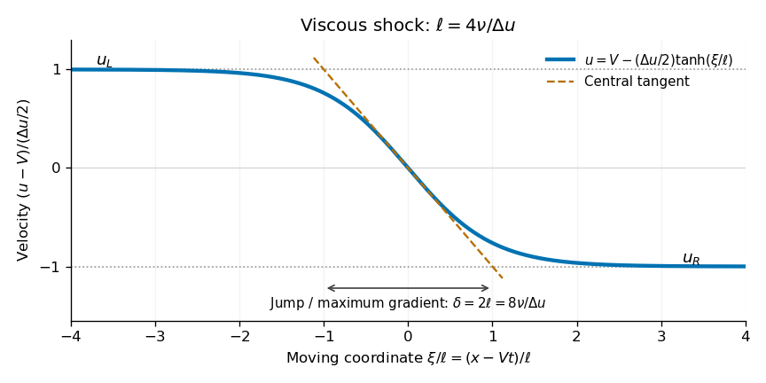
Calculated travelling shock profile and its tangent width; the horizontal coordinate moves with the shock
. Details. 
Treat the cylinder as infinitely long, with a vacuum exterior and no surface tension. Let be its gravitational potential. Integrating the gravitational Poisson equation over a coaxial cylinder of radius and length , then applying the divergence theorem, givesThus the inward gravitational acceleration is . Hydrostatic equilibrium requiresImpose zero pressure on the free surface, , and integrate inward:This is the hydrostatic self-gravitating incompressible cylinder. Its central pressure is , and the units of the expression are . A nonzero external pressure would add that constant to .
Write total pressure and gravitational potential asHere is the Eulerian perturbation of a fluid variable applied to pressure, while is the corresponding gravitational potential perturbation. They have units and , respectively. The constant interior mass density is .
The Euler equations areSubtract the hydrostatic equilibrium relation and discard terms quadratic in the perturbation. Mass conservation gives incompressible flow, and the gravitational Poisson equation has no bulk density perturbation. Thus, strictly inside the fluid,The last equation is Laplace equation, not a statement that self-gravity has disappeared. The displaced surface carries a first-order surface mass density , where is its radial displacement, and this supplies the source and matching conditions for at the moving interface. The axisymmetric gravitational potential of a displaced cylindrical interface, expressed using modified Bessel functions, incorporates that boundary source.
It is useful to define . Taking the divergence of the momentum equation gives . For an axisymmetric Fourier mode with axial wavenumber , regularity at selects radial dependence , the Modified Bessel function of the first kind, since is singular there. In what follows can always be chosen nonnegative.
Use complex amplitudes and take their real parts at the end. Write the radial surface displacement as and the combined potential asThe linear kinematic boundary condition is . Differentiate it once more in time and use the radial momentum equation, , evaluated at the unperturbed radius :With , the mode amplitudes therefore satisfyThe prime differentiates the Modified Bessel function of the first kind with respect to its dimensionless argument, rather than with respect to . The result has units , as required because is a potential. It applies to ; the uniform limit requires separate treatment.
The vanishing total pressure must be imposed at the displaced free surface, not at fixed . The first-order Taylor expansion isSince and , the Lagrangian pressure perturbation condition isThe supplied gravitational perturbation and the combined potential, evaluated at , then giveHere is the Modified Bessel function of the second kind. Equating mode amplitudes and using part (c) yieldsRearrange to obtain the dispersion relation for the axisymmetric gravitational instability of an incompressible cylinder:Every quantity on the right is dimensionless, consistent with having units . The stabilizing term comes from displacing the background hydrostatic pressure profile; omitting the Lagrangian pressure perturbation would lose it.
Define the dimensionless right-hand side of part (d) by . Then . Because and for , its sign is the sign of . The original plot is positive for sufficiently long wavelengths and negative at short wavelengths; the nonzero crossing is approximately . Numerically solving the displayed equation gives .
For , . Write with . The time factor then contains an exponentially growing solution. For , and the ideal inviscid modes oscillate stably, without damping. At the crossing the frequency is zero and the mode is marginal. In terms of the axial wavelength ,The growth rate tends to zero as , so the very longest wavelengths are not the fastest growing. The source plot has its maximum near , corresponding to and . Thus a characteristic fragmentation spacing is several cylinder diameters; a quantitative nonlinear fragment mass is beyond this linear stability calculation.
For unstable modes the physical displacement must be interpreted as with complex amplitudes handled consistently throughout. The paper's real-part notation is harmless for the squared dispersion relation, but it should not be read as imposing real in a gravitational instability calculation. The exactly uniform mode is excluded from the finite- derivation; the limit of the curve alone does not establish a separate volume-preserving uniform-radius mode.
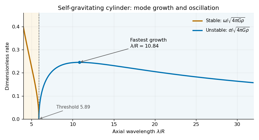
Rates computed from the cylinder dispersion relation as a function of wavelength, showing stable oscillation and unstable growth
. Details. 
The first argument mixes a material fluid element with a fixed spatial volume. For a material volume element following the fluid, its volume is generally time dependent:Therefore the material derivative cannot be taken outside the product with as in the proposed cancellation. Instead, mass conservation statesThe momentum balance for a material fluid element, using Newton's second law, is consequentlyFor a fixed control volume, fluid crosses its boundary and carries momentum; a momentum flux term must be included. Its local conservative form is , equivalent to the displayed Euler equations after using the continuity equation. The erroneous equation omits the term needed to convert a material derivative of momentum density into this conservative form.
For the second task, take a homogeneous fluid with constant mass density , prescribed gravitational acceleration , incompressible flow and inviscid flow. Its equations areUnder the replacement , the same velocity solves these equations if , up to a spatially constant pressure offset. This is density scaling invariance of incompressible Euler flow:The comparison assumes the same geometry and compatible velocity or gravitational free surface conditions; an independently specified nonuniform boundary pressure would supply additional information. The gravitational field is taken as prescribed. If the fluid's own self-gravity must be included, its field changes with mass density, so the invariance need not hold. A single freely moving particle's density-independent gravitational acceleration does not justify neglecting that distinction.
A highly conducting solar wind carries the Sun's magnetic field outward by magnetic flux freezing. This can open magnetic field lines that would form closed loops in a static dipole model. Beyond an opening radius , approximate the field as radial. Constancy of the magnetic flux in a fixed solid-angle flux tube gives the radial solar-wind magnetic flux lawwhich decays more slowly than the vacuum magnetic dipole field, proportional to .
For example, if the field becomes radial already near the solar radius , normalizing both estimates to the same field there givesThus a dipole estimate becomes of order , comparable to the stated hundredfold enhancement. More generally, matching dipolar decay inside to radial decay outside givesThis is a plausible scaling explanation, not a determination of the actual opening radius. The magnetic field need not be outward everywhere: opposite-polarity sectors can preserve zero net magnetic flux through a closed surface, consistent with Gauss's law for magnetism. The argument concerns the changed geometry of the field in a flowing plasma, rather than changing the dipole exponent by assumption.
Take the outward wavenumber ; the absolute value in the source makes the two propagation directions equivalent. The phase velocity of the gravity-capillary wave obeysDifferentiate with respect to :The second derivative is positive, and at both ends of the positive- range, so this is the global minimum. The minimum phase speed of a gravity-capillary wave isFor and the supplied surface tension and mass density,The corresponding wavenumber is , giving wavelength . At this minimum, . Thus the group velocity and phase velocity agree for this particular ripple, although they differ for general gravity-capillary waves.
A shock wave forms when a compressive flow steepens or when gas must be decelerated or turned faster than upstream acoustic waves can communicate the change. Astrophysical examples include a supernova remnant sweeping up surrounding gas, a fast stellar wind colliding with ambient material, and supersonic accretion onto an obstacle or onto a dense gas layer. A large Mach number by itself is not sufficient: a uniform supersonic stream need not contain a shock wave.
Choose the shock frame, and denote upstream and downstream normal velocities by . Integrating the local conservation laws over a thin control volume spanning a steady normal shock wave gives equal fluxes on both sides. Mass conservation gives constant mass flux per unit area,Pressure and advected momentum together give the normal momentum flux,For a thin non-radiating layer, with negligible gravitational-potential change across it, conservation of energy gives equal fluxes . A perfect gas has specific enthalpy , soThese are the Rankine-Hugoniot conditions for a perfect gas. Dissipation inside the thin layer produces an entropy increase and selects the physical compressive branch. Efficient radiative cooling would change the energy relation and may instead lead to an isothermal shock.
Take . Let . Mass conservation gives , and normal momentum conservation givesInsert this into the energy condition from part (a):Rearranging and factoring,The root is the unshocked state. The compressive Strong-shock Rankine-Hugoniot conditions instead giveCorrespondingly, and . These relations require and negligible upstream thermal pressure.
Let denote the total flow speeds, keeping the normal components distinct from them. The original diagram measures from the initial wall direction to the shock wave itself. The outgoing velocity is turned by , so it makes angle with the shock.
Resolve each velocity tangent and normal to the oblique shock. Tangential momentum conservation, with nonzero mass flux and no tangential surface force, makes the tangential velocity continuous:The normal flow obeys the strong normal shock wave result from part (b):Divide the second relation by the first to obtainThe approximation is controlled by the upstream normal Mach number , not just by . This distinction matters on the small-angle weak branch in part (d). The angle convention is also important: formulas using the angle to the shock normal instead would interchange sine and cosine.
Rewrite the relation from part (c) asThe angle-addition identities reduce this toFor , the right side lies strictly between zero and one. There are two physically admissible strong oblique-shock angle branches:Both lie between and . They merge when , proving the maximum deflection through a strong perfect-gas shock,For small positive , the formal strong-shock-limit asymptotics areThe weak branch is normally observed for an unconfined supersonic stream turning through a modest compression corner. It has a smaller normal component of upstream velocity, hence a smaller downstream pressure increase; for small turns the downstream flow remains supersonic. The nearly normal strong branch can be selected by suitable downstream pressure conditions, so it is not mathematically forbidden.
The two limits must be ordered honestly. At finite , the weak oblique shock approaches the Mach angle as , rather than zero. The displayed weak-branch asymptotic applies when the large- limit is taken first, or in the overlapping range , where remains valid.
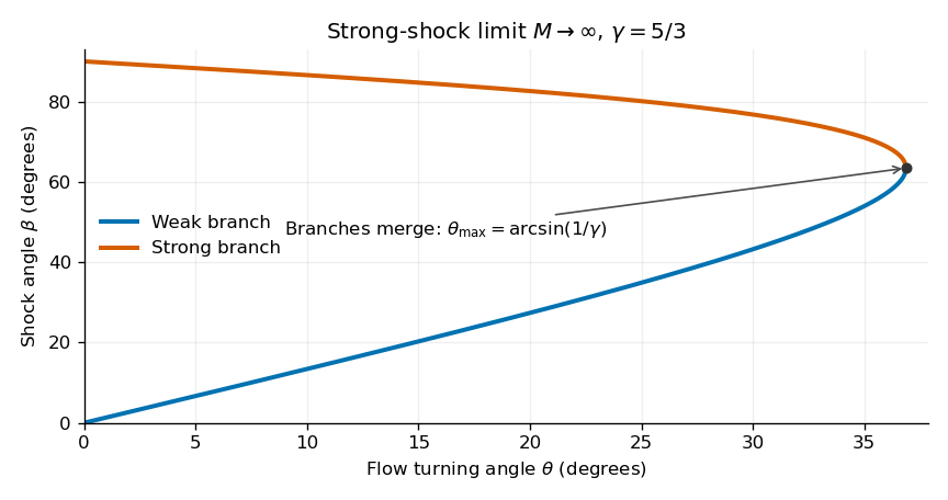
Calculated weak and strong shock-angle branches in the infinite-Mach-number limit, for a monatomic gas
. Details. 
For , , so there is no real solution for an attached straight oblique shock satisfying the assumed geometry. The shock detaches and becomes curved, with a locally strong, nearly normal portion and a subsonic region allowing the flow to adjust to the wall. The precise detached structure depends on the global geometry and downstream conditions; the attached-shock formula cannot be continued to these turns.
Let be the enclosed mass. For spherical symmetry, hydrostatic equilibrium and mass conservation giveThe isothermal equation of state therefore impliesMultiply by , differentiate and eliminate :or equivalently . This is the density equation for an isothermal sphere. Here has units and equals the squared isothermal sound speed.
A regular isothermal sphere does not reach zero density at a finite radius. The finite body discussed later must therefore be truncated by a nonzero external pressure, as in a pressure-confined isothermal sphere. A finite vacuum boundary would not be compatible with this equation of state.
Set and . Then and the equation from part (a) becomesWith , the coefficients cancel, giving the isothermal Lane-Emden equationThe regular central boundary conditions areThe first makes the central mass density equal to . The second follows from smooth spherical symmetry and the vanishing central gravitational acceleration; a preferred radial slope at the origin would be singular. Substitution of a regular power series giveswhich supplies nonsingular starting data for numerical integration. The central conditions select the regular solution, not the singular isothermal sphere.
The particle count is the enclosed mass divided by the particle mass :Integrating the isothermal Lane-Emden equation giveswhere regularity makes the lower endpoint vanish. ThusThe prefactor is a mass divided by a mass, and the remaining factor is dimensionless. In particular, at fixed the dependence on central mass density is , with . Both changes must be retained when comparing equilibria at fixed .
Along a family of equilibria at fixed temperature, and the dimensionless function are fixed. The boundary mass density changes through both and the boundary coordinate :From part (c), , where is constant at fixed temperature and . Set its logarithmic variation to zero:The isothermal Lane-Emden equation gives , so the fixed- relation isSubstitute back into the boundary-density variation:For a nontrivial variation at a finite positive radius, its vanishing gives the fixed-mass turning point of an isothermal sphere:This derivative follows a fixed-mass sequence of equilibria; it is not merely the spatial derivative of density inside one sphere. The corresponding radial variation isAt small , : the boundary density increases while the radius decreases along increasing , giving the stated negative of the stable branch. The first density turning point marks its first loss of radial stability; it need not be confused with a turning point of radius itself.
Using the supplied first critical value , the critical radius of a pressure-confined isothermal sphere isNo radius in metres can be specified without and a central mass density. Here is the isothermal sound speed, consistent with the fixed-temperature variations in part (d). At a given central mass density, equilibria truncated at lie on the first stable branch, while increasing the dimensionless outer radius beyond this first threshold gives an unstable configuration. Numerical integration gives , consistent with the paper's rounded .
For a transparent comparison with the given Jeans length, set the uniform comparison density and use the same speed of sound. ThenBoth scales express the competition between pressure support and self-gravity, with characteristic length . Their numerical closeness under this density choice does not mean that the models impose the same threshold: is a boundary radius, whereas is the wavelength of a perturbation. Comparing with would instead give a factor about . Using the sphere's mean or boundary density instead of its central density changes the coefficient again, so the reference density must always be stated.
The pressure-confined isothermal sphere gives an actual finite, centrally concentrated hydrostatic equilibrium and an explicit confining pressure, making its radial stability threshold more self-consistent for a roughly spherical isothermal cloud. The uniform Jeans instability model gives a simpler local criterion, includes perturbations at different wavelengths, and does not require constructing a spherical equilibrium. Its ideal uniform static infinite background requires the Jeans swindle or an explicitly specified treatment of background gravity. Neither model includes rotation, magnetic fields, turbulent support or a realistic temperature evolution, so neither is a universal collapse criterion.
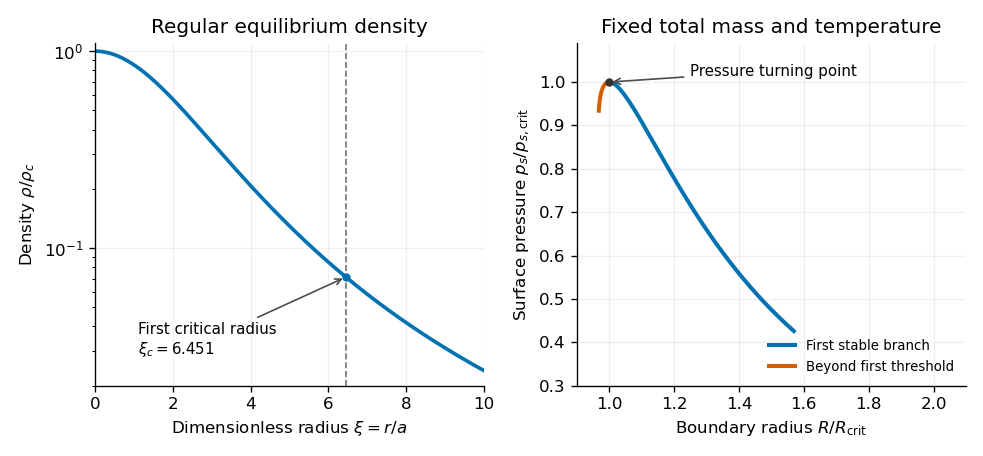
Numerically integrated isothermal-sphere density profile and the first pressure turning point along a fixed-mass sequence
. Details. 
For a steady axisymmetric flow , incompressible flow is automatic. The only material acceleration is centripetal, . The radial Euler equations therefore requireWith no viscosity there is no tangential shear stress to redistribute angular momentum. Any sufficiently regular can therefore be a steady inviscid profile, with the radial pressure adjusted by integrating this equation. This is a statement of equilibrium, not of stability: some such profiles are centrifugally unstable.
For a homogeneous Newtonian fluid with constant kinematic viscosity , assume the same steady purely azimuthal flow. In cylindrical coordinates, the azimuthal Navier-Stokes equation has no pressure forcing or convective term in this state, and becomesEquivalently, , or . Two integrations give the steady circular Couette profile,This is the basic Taylor-Couette flow between rotating cylinders. The constants depend on boundary angular velocities; for radii and prescribed angular velocities ,If the domain includes , regularity requires , leaving solid-body rotation. On an annulus a nonzero is allowed and wall torques maintain the shear.
The restriction concerns a steady profile. An arbitrary initial angular velocity does not cease to exist when viscosity is introduced; within the purely azimuthal ansatz it evolves according to until compatible boundary conditions and angular-momentum constraints determine its long-time state.
Expand the axisymmetric Euler equations about the rotating equilibrium, retaining only terms linear in and in the pressure perturbation. The symbol in this question is the kinematic pressure perturbation,The linearized centripetal term in the radial equation is , after subtracting the equilibrium term . Radial advection of the background azimuthal velocity, together with the cylindrical-coordinate term , givesThis is the azimuthal coupling in the second equation; it also expresses conservation of specific angular momentum for a radially displaced element. The axial equation is acceleration balanced by . Finally, the axisymmetric incompressible flow condition in cylindrical coordinates iswhich expands to the last supplied equation. Background azimuthal advection contributes no term because the perturbations are axisymmetric.
Use the thin-annulus approximation stated in the source, so . LetHere is the conventional Rayleigh discriminant, also the squared local radial epicyclic frequency when positive. For and , the azimuthal and axial mode equations giveThe thin-gap incompressible flow condition then gives . Substitute these into the radial equation:ThusTo put this into exactly the form printed in the paper, defineThe narrow-gap centrifugal stability equation is consequentlyThe two rigid cylinders are impermeable, so the no-penetration boundary condition givesThere is no inviscid no-slip condition on the tangential or axial components.
The sign deserves emphasis: the source's printed plus sign makes its the negative of the conventional Rayleigh discriminant. Using the conventional positive discriminant instead requires a minus sign in front of that potential term. These are equivalent conventions; replacing one without adjusting the other would falsely predict instability of solid-body rotation. The and marginal cases, excluded by these eliminations, must be treated separately or by limits.
Let be a nonzero admissible mode, multiply the equation of part (d) by its complex conjugate and integrate between the cylinders. The endpoint conditions remove the boundary term in integration by parts, giving the Rayleigh stability integral identityRearrange to obtain a real Rayleigh quotient:The denominator is strictly positive. Consequently, with the paper's convention,The weak inequality excludes exponentially growing axisymmetric modes, but permits marginal cases and possible algebraic growth when the restoring effect vanishes. Strict negativity avoids that degeneracy. Equivalently, the conventional Rayleigh discriminant is positive, or the squared specific angular momentum increases outward:This is the Rayleigh centrifugal stability criterion. In the suggested Time-independent Schrödinger equation analogy, a growing mode has ; if , its effective potential is nonnegative. The nonnegative kinetic term and that potential cannot have the required negative eigenvalue , which gives the same exclusion.
As a sign check, for solid-body rotation and . In a gap of width , the radial modes haveas expected for inertial waves. The argument establishes axisymmetric inviscid stability within the stated thin-gap model, rather than a claim about all perturbations of a viscous flow.
Write the initial mass density as . The ideal gas law gives pressure , and the sphere has . Here is the Boltzmann constant and is the gravitational constant. First obtain the gravitational potential energy by adding concentric shells. The mass inside radius is , soIn a small contraction at fixed total mass, the gravitational energy released is . The positive work required against the gas pressure is . Equating these givesUse to eliminate the radius. The uniform-sphere pressure-work collapse criterion isThe units are kilograms: has units , and supplies . At fixed initial and , makes gravity stronger than the pressure-work requirement in this model, allowing contraction.
This is a Jeans mass estimate for homologous contraction of an initially uniform sphere. It is not an exact stability limit for a hydrostatic gas sphere: uniform mass density and uniform temperature would give uniform pressure, rather than the gradient required by hydrostatic equilibrium. The numerical coefficient therefore differs from conventions based on a Jeans instability wavelength or a pressure-confined isothermal sphere. Subsequent contraction also depends on heat exchange; isothermal pressure support during gravitational collapse weakens relative to gravity as the radius decreases.
The exponential factor removes the first spatial derivative. Apply the chain rule explicitly:while . Substituting into the supplied density equation, the terms proportional to cancel, leavingThis is the atmospheric acoustic cutoff transformation. There is a sign error in the target equation in the original PDF, as well as in the transcription: the last term must be for real positive . If the displayed minus sign is retained literally, coefficient matching would require , so it would not define a real characteristic oscillation period.
For the corrected equation, a plane wave has dispersion relationThus is the acoustic cutoff frequency: vertically propagating acoustic waves have . The scale height and sound speed have units metres and metres per second, respectively, so has units .
For an order-of-magnitude estimate in the lower terrestrial atmosphere, take and . These are representative atmospheric values, not additional data specified by the paper. They giveThe isothermal atmosphere approximation is local: a real atmospheric temperature profile and the thermodynamic response of the disturbance modify the precise cutoff and period.
For an inverted free surface, gravity promotes a displacement instead of restoring it. The surface tension term still resists curvature. Hence the gravity-capillary wave relation becomes, with ,For , where , . Writing the displacement as gives the Rayleigh-Taylor instability growth rateShorter wavelengths, , remain oscillatory because surface tension dominates. The marginal scale is determined by the capillary length,A sufficiently small aperture excludes the long unstable modes: this is finite-aperture stabilization of an inverted liquid surface. The estimate requested is therefore a container opening of order one centimetre, with the marginal full wavelength rather than a geometry-independent maximum diameter.
The exact largest opening cannot be fixed from the stated infinite-surface dispersion relation alone. It requires the aperture shape and contact-line boundary conditions. For example, a one-dimensional span of width whose contact line is pinned at both ends has a half-sine lowest mode with . In that simple model,Different geometries change the numerical factor. This is a small-disturbance stability estimate with negligible air inertia and no leakage or contact-line failure; a guarantee that a real inverted container retains its water needs those additional boundary details.
Following a fluid element. Let be a pathline, satisfying . The material derivative, also called the Lagrangian time derivative, is the rate observed while following that element. The multivariable chain rule givesThe partial derivative holds position fixed; the advection term accounts for motion through a spatially varying field. For a vector field, the same formula applies component by component in fixed Cartesian axes.
Momentum balance. For an inviscid flow, pressure is the only surface stress. A small material volume has net pressure force , obtained by the divergence theorem. Its mass is and its material acceleration is . Applying Newton's second law gives the Euler equations for an inviscid fluid,This is the local momentum conservation equation when viscosity and physical body forces are absent. A prescribed body force per unit mass would add on the right.
Changing to rotating coordinates. In a rotating frame with constant angular velocity , the lab acceleration is the rotating-frame material acceleration plus . ThereforeFor uniform rotation,With constant , this gives the Euler equation in a uniformly rotating frame,The term subtracted from is the equilibrium centrifugal contribution. Dividing the bracket by defines a reduced pressure , with units . The Coriolis acceleration remains a velocity-dependent term.
Linear disturbances. Linearize about rest in the rotating coordinates, with the equilibrium part of removed. The advective acceleration is quadratic in disturbance amplitude, so the linearized Euler equations and incompressible flow condition areTaking the curl removes the pressure gradient. The identitygives the inertial-wave vorticity equation,
Plane-wave frequencies. Let and use the given plane wave convention. Incompressible flow requires , and the vorticity equation givesFor a nonzero frequency, apply again, using . It follows thatThis is the inertial-wave dispersion relation. If is the angle of the wavevector to the rotation axis, the positive angular frequency is . It is largest, , for a parallel wavevector, decreases to zero for a perpendicular one, and is independent of the magnitude of the wavenumber at fixed direction. The two signs describe the two oscillatory polarization branches. When , the zero-frequency result is obtained directly from the linear equations rather than by dividing by ; it describes the nonoscillating balanced limit.
The local conservation laws. The first equation is the radial Euler equation: the material acceleration is caused by the pressure gradient force per unit mass, . It neglects gravity and viscosity. The second equation is mass conservation in spherical coordinates,The term appears because the area of a spherical surface grows as .
To obtain the third equation, let be the specific internal energy of an ideal gas with constant heat capacity ratio . The first law of thermodynamics for a smooth adiabatically moving element isDifferentiating and collecting terms givesand henceThus the entropy parameter is conserved along each smooth pathline; for fixed composition, specific entropy differs from only by a constant. This is local isentropic flow behind the shock. A physical shock wave itself generates entropy and must be treated with jump conditions, rather than by applying this smooth equation across the discontinuity.
The front-radius scaling. In the self-similar blast wave approximation there is no scale set by ambient pressure, cooling, gravity, or the initial source radius. Write . Using and , dimensional analysis givesThus , , andThe dimensionless coefficient depends on and the resolved similarity profiles; dimensions alone do not fix it. Define the length scale , so and the front is at the fixed coordinate .
Kinetic energy. Substitute and into the volume integral. Since and ,But , so the first of the spherical blast-wave similarity energy integrals isThe conclusion requires a fixed, integrable similarity profile, as in the finite-energy blast solution. Expansion increases the swept-up mass while reducing the characteristic squared speed, leaving this product constant.
Pressure and internal energy. The derivatives of the similarity variable areWriting a prime for differentiation with respect to , the material acceleration becomesThe radial momentum equation therefore requires a pressure gradient on the scale . Integrating over radius gives pressure similarity in a spherical blast wave:whereThe prefactor has units , as required for pressure. Strictly, the momentum equation alone permits an additional pressure uniform in space and arbitrary in time. In the scale-free strong-blast solution, shock matching and the remaining thermodynamic equation fix that freedom with the same similarity scaling; any allowed constant of integration is included in . An independently imposed external pressure would introduce another scale and invalidate the simple dimensional ansatz.
For constant , the internal energy is consequentlyIf is the total excess explosion energy, its normalization isThe two constant fractions need not be equal. No explicit solution for is needed to establish their time independence.
Hydrostatic equilibrium with self-gravity. A resting fluid obeys . Spherical symmetry and the Poisson equation for Newtonian gravity giveEliminate the Newtonian gravitational potential derivative to obtainEquivalently, the shell theorem gives and , which leads to the same hydrostatic equilibrium equation.
A uniform-density liquid. With constant , . There is no central point mass, so the interior gravitational acceleration magnitude is . ThusUse at a vacuum boundary, neglecting surface tension. The uniform-density planetary pressure profile isThe central value can also be writtenIt has units pascals and decreases smoothly from its maximum at the centre to zero at the surface.
An isothermal gas. Here is the constant isothermal sound speed, with . Try , so . The two sides of the equilibrium equation becomeThus , giving the singular isothermal sphere,This does not describe a finite gaseous sphere in vacuum. Both pressure and mass density diverge at the centre, and for every finite outer radius , so it cannot meet there. Extending it to infinity removes the finite-radius pressure jump but makes the total mass infinite. It is useful as an idealized profile over an intermediate radial range, or as a truncated model with nonzero external pressure. The vacuum boundary obstruction for an isothermal sphere also applies to the regular, nonsingular isothermal solution; removing the central singularity does not produce a finite vacuum surface.
Steady outflow. In the wind calculation, take the central mass to be fixed and neglect the wind's own self-gravity. Constant mass flow rate and the isothermal equation of state giveThe steady radial Euler equation isSubstituting the density derivative givesThis is the isothermal Parker wind equation. A smooth sonic point requires both sides to vanish when , soMaintaining constant temperature during expansion generally requires heat input; it is an isothermal model, not the adiabatic blast-wave model of Question 5.
The escaping branch at large radius. Integrate the wind equation, using dimensionless logarithm arguments:Set and . ThenFor the accelerating transonic branch, , which fixes . At on its supersonic branch, and is smaller than . ConsequentlyA first correction makes the ordering explicit:This is the large-radius asymptotics of an isothermal Parker wind. The leading expression also holds for other supersonic branches with finite .
The source implicitly selects an escaping wind. Positive steady outward flow alone does not determine that branch: a subsonic isothermal breeze also satisfies the differential equation. Its limit gives , hence and . Such a breeze needs nonzero pressure at infinity. Selecting a regular outflow from a subsonic base into vanishing ambient pressure instead gives the accelerating transonic wind used above.
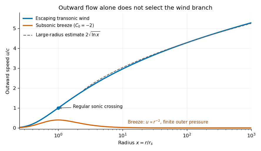
Original numerical branches of the integrated isothermal wind equation, showing the escaping wind, its logarithmic asymptote, and a pressure-confined subsonic breeze
. Details. 
The asymptotic speed has the same units as ; the logarithm is dimensionless. Its unlimited growth is a formal feature of indefinite isothermal heating and a prescribed point-mass potential. Real heating, surrounding pressure, and eventually the neglected wind mass limit that extrapolation.
Articles were limited to the first 100 out of 147 total.
Articles by others on the same topic
There are currently no matching articles.