Interdisciplinary paper IDP1 (Atmospheric Chemistry and Global Change)

Solution

A small global warming potential requires both a small greenhouse gas radiative efficiency per unit emitted mass and a short atmospheric lifetime. Weak absorption in the terrestrial atmospheric window is desirable, particularly where absorption by existing gases is weak; strong carbon–fluorine vibrational bands can make even an ozone-safe substitute an efficient greenhouse gas. Rapid removal by lower-atmospheric chemistry limits the integrated burden, provided it does not generate abundant, long-lived radiatively active products. The atmospheric residence time and the absorption spectrum must therefore be assessed separately.

b

Solution

In a vertical-beam, effective-wavelength Beer-Lambert law approximation, the optical depth above altitude

z

τ (z) = σ_{O_{2}} N_{O_{2}} (z) + σ_{O_{3}} N_{O_{3}} (z)

. Using centimetres consistently gives

τ_{20} = 1.50 + 12.60 = 14.10, τ_{40} = 0.084 + 0.340 = 0.424.

The transmitted photon flux is proportional to

e^{- τ}

. If the parent-gas absorption cross section and photodissociation yield are otherwise the same, they cancel in the ratio of photolysis rate coefficients:

\frac{J ( 40 km )}{J ( 20 km )} = e^{τ_{20} - τ_{40}} = e^{13.676} = 8.70 \times 1 0^{5} .

The corresponding fractions of the unattenuated beam are about

7.52 \times 1 0^{- 7}

and

0.654

. Strong shielding by the overlying oxygen and especially ozone therefore makes destruction vastly faster higher in the stratosphere, even though the molecular absorption properties have not changed.

This numerical ratio uses the intended simplified radiation model. A real photolysis rate coefficient integrates wavelength-dependent actinic flux, absorption cross section and quantum yield. A nonvertical direct beam would use slant optical depth

τ / cos θ

; diffuse scattering and the true solar spectrum would also matter. The supplied effective cross sections do not specify a unique broadband radiative-transfer calculation.

c

Solution

The global warming potential compares equal-mass pulses, while the tabulated greenhouse gas radiative efficiencies are per ppb. For a fixed emitted mass, the initial mixing ratio is inversely proportional to molar mass. The molecular formulas give approximately

M_{r} = 151.39 g mo l^{- 1}

for

C_{2} H_{2} C l_{3} F

and

M_{11} = 137.36 g mo l^{- 1}

for

CC l_{3} F

. Thus the ratio of mass-based greenhouse gas radiative efficiencies is

(0.24/0.26) (M_{11} / M_{r})

In the standard one-box interpretation, the two quoted removal times represent independent first-order sinks acting on the burden. Their rates add, giving

τ_{r}^{- 1} = τ_{trop}^{- 1} + τ_{strat}^{- 1}, τ_{r} = (\frac{1}{0.75} + \frac{1}{20})^{- 1} = 0.72289 yr .

For exponential pulse removal, the time-integrated abundance is proportional to

τ (1 - e^{- H / τ})

. Dividing the replacement's forcing integral by the CFC-11 integral cancels the unknown carbon-dioxide reference integral:

GWP_{100, r} = 5160 \frac{0.24}{0.26} \frac{137.36}{151.39} \frac{0.72289 ( 1 - e ^{- 100/0.72289} )}{55 ( 1 - e ^{- 100/55} )} ≃ 67.8 ≃ 68.

The finite-horizon factor for CFC-11 is important:

1 - e^{- 100/55} = 0.8377

, not one. Omitting the molar-mass correction would incorrectly compare equal-ppb rather than equal-mass pulses.

This is about 76 times smaller than the stated CFC-11 value, because rapid tropospheric removal outweighs the fairly similar per-ppb greenhouse gas radiative efficiencies. It still represents appreciable warming per emitted mass. If the shorter lifetime alone is used as the troposphere-dominated approximation, the result is

GWP_{100} ≃ 70.4

, close to the combined-rate result. If the two given lifetimes instead describe separate local compartments, an exact two-box calculation would also require exchange rates and burden partitioning; those are not supplied. The boxed result states the usual one-box assumption explicitly.

d

Solution

TODO: user-deferred biological component. Biological carbon uptake, storage and release are outside the current scope. The physical and ocean-chemistry explanation is given here; the deferred component means this is not a complete all-process answer.

There is no single first-order atmospheric lifetime for an added carbon dioxide pulse. Air–sea gas exchange and adjustment of the surface mixed layer act on years-to-decades scales; redistribution into the ocean interior takes centuries to millennia. These transfers partition carbon between atmosphere and ocean rather than making the entire added carbon inventory disappear. Dissolution also changes the ocean's carbonate speciation: conversion among dissolved carbon dioxide, bicarbonate and carbonate buffers the uptake, but provides a finite capacity at a given alkalinity. A substantial perturbation therefore remains airborne after the faster exchanges have adjusted.

Further removal involves dissolution of carbonate sediments and carbonate compensation over several thousand years, followed by the much slower silicate-weathering and burial pathway, typically tens to hundreds of thousands of years. The exact fractions and times depend on pulse size and model conditions. A thousand years exceeds the fast exchange times but not the complete ocean–solid-Earth adjustment time, so a residual atmospheric perturbation is expected. An intercomparison found a substantial long tail after ocean equilibration, with further carbonate neutralization on roughly 3–7 kyr scales.^[ref]

e

Solution

For a gas whose lifetime is much less than the selected horizon, the numerator of its global warming potential has nearly saturated:

\int_{0}^{H} a_{i} m_{i} (t) d t ≃ a_{i} m_{i} (0) τ_{i}

. The carbon-dioxide denominator continues to accumulate because of its long-lived response. Consequently a shorter horizon usually gives a larger GWP for this short-lived substitute; a longer horizon gives a smaller GWP. If the horizon becomes comparable to, or shorter than, the substitute's lifetime, the numerator also depends strongly on the horizon and cannot be replaced by its infinite-time limit.

The horizon is a value choice, and integrated forcing is not the same as temperature at a chosen future date. Equal-GWP pulses can therefore have different near-term warming and long-term temperature paths. The result also depends on greenhouse gas radiative efficiency, background concentrations, lifetime estimates and which indirect chemical effects or feedbacks are included. A pulse-based metric does not by itself describe a continuing emissions trajectory, nor does it measure ozone depletion or local air-pollution impacts. Comparisons should state the horizon, the emission scenario and the chosen climate outcome.^[ref]

2

a

Solution

Take a fixed amount of dry air, with no phase change, moving quasistatically so that its pressure matches the surrounding atmosphere. From the first law of thermodynamics and

H = U + p V

d H = d U + p d V + V d p = d q + V d p .

For adiabatic motion

d q = 0

. Treating the parcel as an ideal gas of fixed composition makes its enthalpy depend only on temperature, so for

n

moles

d H = n C_{p} d T

even though the pressure changes. Hence

n C_{p} d T = V d p

. The environment is in hydrostatic equilibrium,

d p / d z = - ρ g

, and the parcel is taken to have the ambient density at the displacement point. Using

ρ = n M / V

gives

n C_{p} \frac{d T}{d z} = V \frac{d p}{d z} = - n M g, \frac{d T}{d z} = - \frac{M g}{C _{p}} = - \frac{g}{c _{p}} .

Here

C_{p}

is molar and

c_{p} = C_{p} / M

is mass-specific heat capacity. Positive

z

points upward; the commonly quoted positive dry adiabatic lapse rate is

Γ_{d} = - d T / d z

. Approximate constancy of

g

and heat capacity gives a constant gradient. Condensation, external heating, entrainment or composition changes invalidate this dry-parcel relation.

b

Solution

Convert the molar mass to

0.0288 kg mo l^{- 1}

before substitution:

\frac{d T}{d z} = - \frac{( 0.0288 ) ( 9.81 )}{29} = - 9.742 \times 1 0^{- 3} K m^{- 1} ≃ - 9.74 K k m^{- 1} .

The often-used environmental value near

- 6.5 K k m^{- 1}

is less steep because rising moist air can condense water vapor, releasing latent heat and offsetting some expansion cooling. A saturated parcel therefore follows a smaller-magnitude moist adiabatic lapse rate, which varies with temperature, pressure and water content. Real environmental profiles also reflect radiation, mixing and weather systems;

6.5 K k m^{- 1}

is a representative profile value, not a universal parcel law.

c

Solution

Much stratospheric heating is supplied by absorption of solar ultraviolet radiation by oxygen and ozone, whereas carbon dioxide is an important emitter of thermal infrared radiation. In the usual stratospheric balance, increasing carbon dioxide enhances net infrared cooling at the original temperature without supplying a matching increase in the solar heating. Temperature must fall until infrared emission and absorption again balance the heating.

A useful optically thin schematic is

Q_{solar} = c_{C O_{2}} K [B (T) - \overline{J}]

, where

B (T)

represents the relevant thermal source function and

\overline{J}

the incident infrared radiation field. With positive fixed solar heating and an approximately fixed radiation field, increasing

c_{C O_{2}}

lowers the required

B (T) - \overline{J}

, hence lowers

T

. This explains why the surface greenhouse argument cannot simply be applied locally to the stratosphere. Spectral blocking of upwelling radiation contributes too; the real response depends on altitude, ozone heating and radiative transfer, rather than emissivity alone.^[ref]

d

i

Solution

Put

X = [O_{3}]

and

u = T^{- 1}

. The fast oxygen–ozone partition obeys

k_{4} [O] [O_{2}] [M] = J_{5} X, [O] = \frac{J _{5} X}{k _{4} [ O _{2} ] [ M ]} .

Dividing the production–loss balance by two and substituting gives

P = A X^{2} + BX, P = J_{1} [O_{2}], A = \frac{k _{2} J _{5}}{k _{4} [ O _{2} ] [ M ]}, B = k_{3} [NO] .

Under the specified restriction, all temperature dependence lies in the three rate coefficients: hold the photodissociation rates and the concentrations of

O_{2}

M

and NO fixed. Then

d ln A / d u = - 2100 - 510 = - 2610 K

and

d ln B / d u = - 1200 K

. Defining

Y = d ln X / d u

, differentiation yields

0 = A X^{2} (- 2610 + 2 Y) + BX (- 1200 + Y) .

(3)

Therefore

\frac{d ln [ O _{3} ]}{d ( T ^{- 1} )} = \frac{2610 L _{C} + 1200 L _{N}}{2 L _{C} + L _{N}}, L_{C} = k_{2} [O] [O_{3}], L_{N} = k_{3} [NO] [O_{3}] .

(4)

The factor two in the denominator multiplying

L_{C}

comes from the additional dependence

[O] \propto X / k_{4}

; ignoring that dependence would give the wrong sensitivity. This derivative has units of kelvin.

ii

Solution

Using the stated loss ratio

L_{N} = 3 L_{C}

in the derived logarithmic sensitivity gives

\frac{d ln [ O _{3} ]}{d ( T ^{- 1} )} = \frac{2610 + 3 ( 1200 )}{2 + 3} = 1242 K .

The positive sign means that cooling, which increases

T^{- 1}

, increases the steady ozone concentration within this restricted middle-stratosphere model.

iii

Solution

The change in inverse temperature is

Δ u = 1/290 - 1/300 = 1.14943 \times 1 0^{- 4} K^{- 1}

. Treating the sensitivity as approximately constant over the interval,

Δ ln [O_{3}] ≃ 1242Δ u = 0.142759, \frac{[ O _{3} ] _{290}}{[ O _{3} ] _{300}} ≃ e^{0.142759} = 1.15345.

Thus the predicted concentration increases by about 15.3%. Linearizing the exponential gives a rougher 14.3% estimate; a logarithmic change is not itself the exact fractional change.

An independent finite-change calculation checks this approximation without keeping the loss ratio artificially fixed. Normalize the initial Chapman and nitrogen-cycle loss terms to 1 and 3, so the initial production is 4. If

r = X_{290} / X_{300}

, the new steady balance is

e^{- 2610Δ u} r^{2} + 3 e^{- 1200Δ u} r = 4

. Its positive root is

r = 1.15342

, essentially the same result.

e

Solution

Lower winter temperatures favour formation and persistence of polar stratospheric clouds, providing particle surfaces on which reservoir chlorine can be activated, for example

HCl + ClON O_{2} ⟶ C l_{2} + HN O_{3}, HCl + HOCl ⟶ C l_{2} + H_{2} O .

These are heterogeneous surface processes; cooling changes particle abundance, adsorption, phase and reaction uptake, so a simple gas-phase Arrhenius argument is insufficient. Removal of nitric acid in sedimenting particles can also delay conversion of active chlorine back into chlorine nitrate. The relevant condensation thresholds depend on pressure and water/nitric-acid abundances, rather than a single universal temperature.

Once sunlight is present,

C l_{2} + h ν \to 2Cl

provides active chlorine. In the chlorine monoxide dimer cycle,

2 (Cl + O_{3} ClO + ClO + M ClOOCl + h ν ClOO + M ⟶ ClO + O_{2}), ⇌ ClOOCl + M, ⟶ Cl + ClOO, ⟶ Cl + O_{2} + M .

The net reaction is

2 O_{3} \to 3 O_{2}

, with chlorine regenerated. Low temperature favours formation of the ClOOCl dimer and suppresses its thermal dissociation, making photodissociation rather than thermal return of two ClO radicals more competitive. Laboratory flow experiments formed the dimer at 220–240 K and distinguished its infrared and ultraviolet signatures, supporting the chemical identity needed for this mechanism.^[ref]

Colder polar conditions can prepare and sustain greater springtime ozone loss, but darkness alone does not drive the photolytic cycle. In polar night reactive precursors can accumulate; sunlight is required for rapid dimer-cycle ozone destruction. This differs from the middle-stratospheric gas-phase cooling response derived above.^[ref]

3

a

Solution

Photodissociation of nitrogen dioxide forms an oxygen atom, followed by third-body recombination:

N O_{2} + h ν \to NO + O, O + O_{2} + M \to O_{3} + M .

If NO is converted back to nitrogen dioxide only by

NO + O_{3} \to N O_{2} + O_{2}

, this is a null cycle with no net ozone production. Oxidation of a volatile organic compound by OH generates organic peroxy radicals, and often hydroperoxyl radicals, which instead oxidize NO without consuming ozone:

R O_{2} + NO \to RO + N O_{2}, H O_{2} + NO \to OH + N O_{2} .

The newly formed nitrogen dioxide can then photolyse, giving net ozone production. These chain reactions require sunlight, radical production and both precursor families.

In an NOx-limited ozone-production regime, NO is too scarce for efficient peroxy-radical conversion; competing peroxide-forming radical termination becomes important. Reducing nitrogen-oxide emissions then reduces ozone production. In a VOC-limited ozone-production regime, plentiful nitrogen oxides remove OH through

OH + N O_{2} + M \to HN O_{3} + M

, so organic oxidation and radical supply are limiting. Reducing volatile-organic emissions is effective there, while a modest nitrogen-oxide reduction can initially increase ozone by reducing radical termination and NO titration. Sufficiently large nitrogen-oxide reductions can move the system into the limited regime and eventually lower ozone. The appropriate control therefore depends on the chemical regime and the regional transport history, not merely the largest local emission. The ozone isopleth diagram below uses an explicitly schematic response function to show derivative signs, not a fitted concentration or emissions-control prediction.^[ref]

Figure 1.
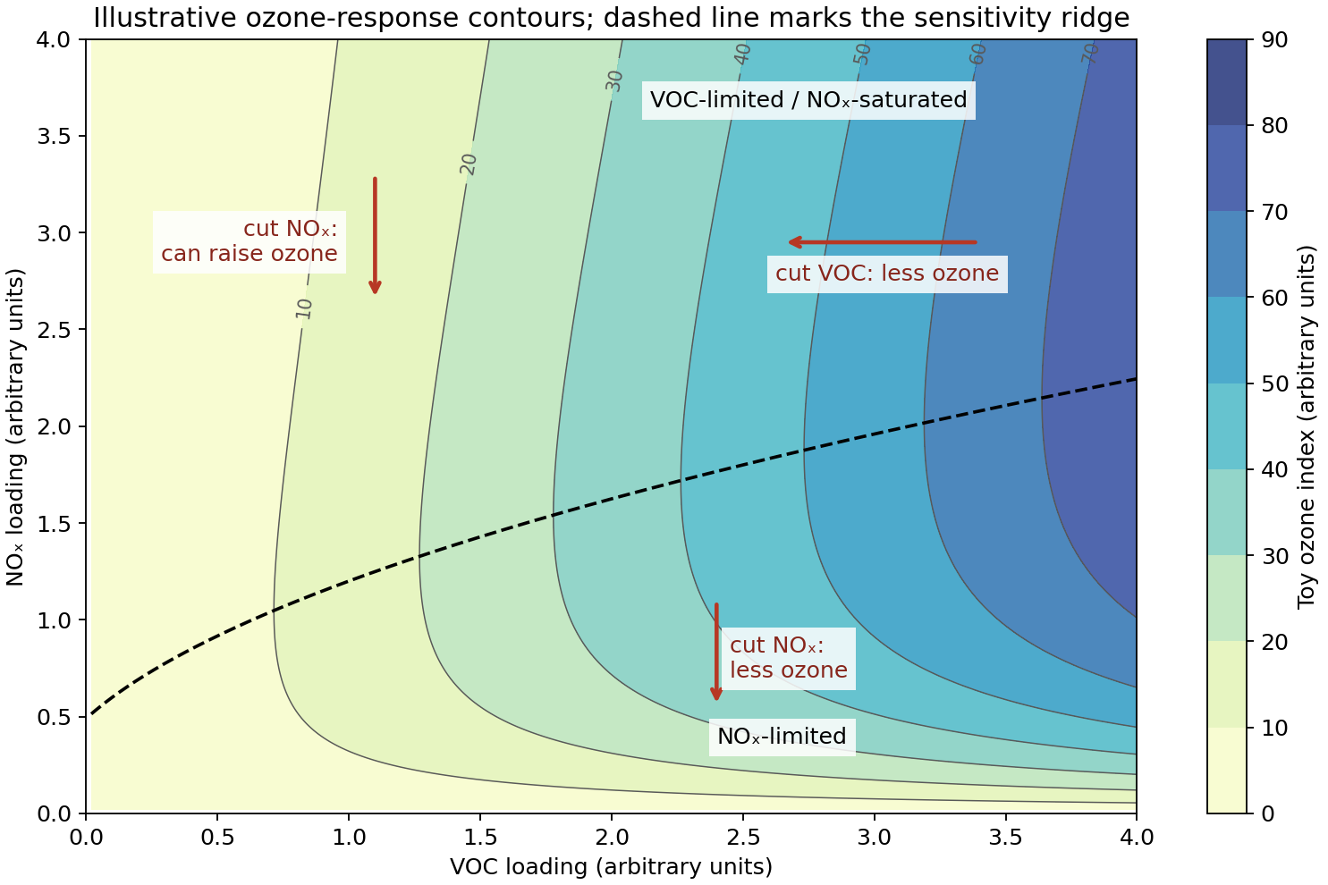
Original schematic showing opposite local ozone responses to nitrogen-oxide controls in two chemical regimes
. **Details**.

b

i

Solution

The profile shows a low-ozone mixed layer up to approximately 2 km, with roughly 30 ppb ozone, and an overlying free-tropospheric value of roughly 50 ppb. The rise occurs through a transition layer extending to about 2.8 km, so these are approximate regime readings, not exact values for every altitude. The horizontal axis is already a mixing ratio; it does not provide a number density without additional air-density information.

ii

Solution

Excited

O (^{1} D)

has two competing fates. Collisional deactivation returns ground-state oxygen, which reforms ozone rapidly; reaction with water instead gives net ozone loss and two OH radicals. The chemical branching fraction for the latter is

f_{w} = \frac{k _{3} [ H _{2} O ]}{k _{2} [ M ] + k _{3} [ H _{2} O ]} = \frac{3.30 \times 1 0 ^{7}}{6.38 \times 1 0 ^{8} + 3.30 \times 1 0 ^{7}} = 0.0491803.

Thus only about 4.92% of these ozone photolyses directly lead to the specified net chemical loss; treating every photodissociation as permanent removal would overestimate the sink. The corresponding first-order rate is

J_{1} f_{w} = 9.8361 \times 1 0^{- 7} s^{- 1}

. Converting the given hydroperoxyl mixing ratio to a concentration gives

[H O_{2}] = 20 \times 1 0^{- 12} [M] = 4.4 \times 1 0^{8} c m^{- 3}

, so

k_{4} [H O_{2}] = 9.6800 \times 1 0^{- 7} s^{- 1}

For a well-mixed marine atmospheric boundary layer of depth

H = 2 \times 1 0^{5} cm

, the downward surface flux is

v_{dep} [O_{3}]

. Dividing by the layer volume per unit area gives a first-order dry deposition rate

v_{dep} / H = 7.5 \times 1 0^{- 7} s^{- 1}

. The air density cancels on expressing the entire balance in ozone mixing ratio

χ

\frac{d χ}{d t} = P_{χ} - (J_{1} f_{w} + k_{4} [H O_{2}] + \frac{v _{dep}}{H}) χ .

At steady state, with

P_{χ} = 0.25/3600 ppb s^{- 1}

χ_{O_{3}} = \frac{0.25/3600}{2.70161 \times 1 0 ^{- 6}} = 25.7 ppb .

(3)

The effective removal time is about 4.28 days. This calculation assumes a uniform layer of the diagnosed depth, fixed chemical conditions and a local time-independent balance.

iii

Solution

The observed value is about 4 ppb higher than the local chemical–dry deposition balance predicts. Entrainment from the ozone-richer free troposphere adds a term

(w_{e} / H) (χ_{FT} - χ_{BL})

; horizontal Advection can likewise import ozone or longer-lived precursors from other regions. Time dependence, including the day–night cycle of photodissociation and changes in mixing depth, is also omitted. The approximately four-day model adjustment time means that air arriving at the measurement location need not have attained the assumed local steady state. These transport and history terms can raise ozone without changing the given local chemical constants.

c

Solution

For a liquid cloud at fixed water content and geometrical thickness, more cloud condensation nuclei can produce more, smaller droplets. The increased total extinction area raises optical depth and reflected sunlight: the Twomey effect gives negative shortwave radiative forcing. It is an indirect aerosol effect mediated by cloud microphysics, rather than direct aerosol scattering.^[ref]

Smaller droplets can also delay collision-coalescence and drizzle, potentially increasing liquid-water retention, cloud lifetime or coverage; that adjustment would usually strengthen cooling for low reflective clouds. It is not universal: evaporation and mixing with dry air can reduce water content or cloud cover, and dynamical changes can oppose the simple lifetime argument. Absorbing particles can heat an atmospheric layer, sometimes evaporating cloud and producing a positive semi-direct forcing, but their vertical position can instead stabilize a cloud layer and reverse the response. Aerosols can additionally alter ice nucleation and mixed-phase precipitation, with no single forcing sign independent of cloud type. The net response combines shortwave reflection and longwave thermal effects, and depends on cloud height, optical depth and adjustments. Thus the fixed-water Twomey sign is robust within its assumptions; adjustment and ice-cloud signs require context.^[ref]

d

i

Solution

Hold liquid-water content and cloud thickness fixed, as required for a partial sensitivity to droplet number. Then

τ = K N_{d}^{1/3}

, so

d τ / d N_{d} = τ / (3 N_{d})

. Differentiating the albedo relation gives

d A / d τ = 7/ (τ + 7)^{2}

, hence

\frac{d A}{d N _{d}} = \frac{7 τ}{3 N _{d} ( τ + 7 ) ^{2}} .

Since

A = τ / (τ + 7)

and

1 - A = 7/ (τ + 7)

\frac{d A}{d N _{d}} = \frac{A ( 1 - A )}{3 N _{d}} .

The factor

A (1 - A)

peaks at

A = 1/2

, so the albedo response to a fixed fractional droplet-number change is greatest at intermediate albedo and weaker near either saturation limit.

ii

Solution

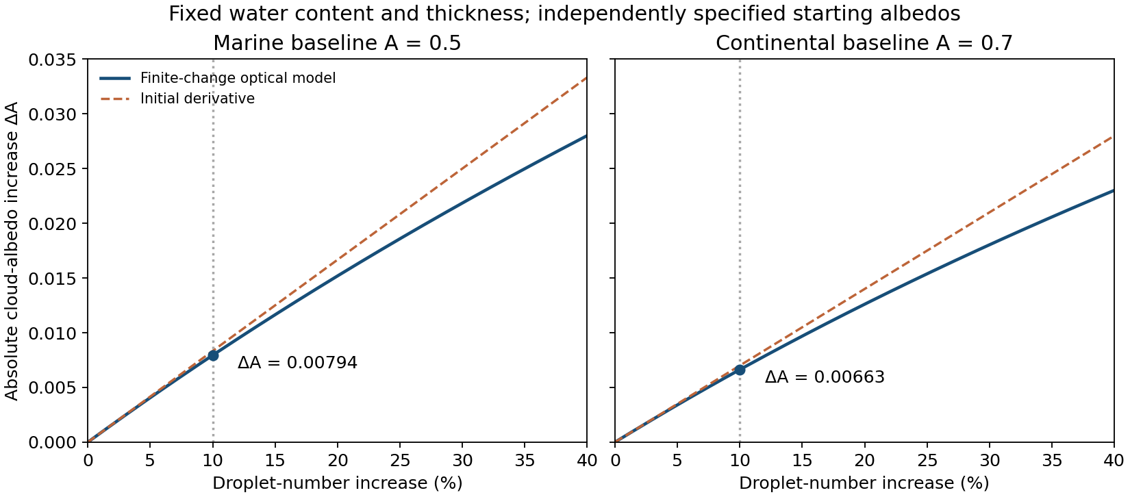
For a small fractional change

ϵ = Δ N_{d} / N_{d}

, use

Δ A ≃ A (1 - A) ϵ /3

. With

ϵ = 0.1

the changes are

Δ A_{marine} ≃ 0.00833, Δ A_{continental} ≃ 0.00700.

Thus the respective albedos become approximately 0.5083 and 0.7070 in the first-order calculation. These are increases of 0.83 and 0.70 percentage points, not 0.83% and 0.70% relative changes. Relative to the initial albedos, the increases are about 1.67% and 1.00%.

The exact finite-change version of the stipulated optical model is

A^{'} = s A / (1 - A + s A)

with

s = (1.1)^{1/3}

, giving

A_{marine}^{'} = 0.50794

and

A_{continental}^{'} = 0.70663

. Its slightly smaller changes are consistent with curvature neglected in the differential approximation. For equal fractional number increases, the cleaner, intermediate-albedo marine cloud is somewhat more susceptible; for equal absolute number increases its susceptibility would be much greater because of the extra

1/ N_{d}

factor. The two starting albedos are treated as the supplied separate baselines, not as an exact common-proportionality calibration of the approximate optical-depth law.

Figure 1.
Original finite-change and tangent predictions for the two specified cloud-albedo baselines
. **Details**.

iii

Solution