Source: public Oxford archive. The held cover dates this sitting to 12 September 2013. All four Section B options are answered.
Near zero, the Taylor expansions areThe constant, linear and quadratic terms cancel in the numerator. ConsequentlyThe square root and logarithm are both real in a sufficiently small neighborhood of zero, so the two-sided real limit is well defined.
Use the outward normal vector. The vector field is , with divergence . By the divergence theorem, its outward flux equals the integral of this divergence over the solid cylinder. Each horizontal slice has area , soFor an independent boundary check, the cylindrical side contributes , the top contributes , and the bottom contributes zero. Their sum is again . Reversing all normals changes its sign.
For one sine mode, and . The wave equation on a string therefore holds whenThe superposition principle gives the same equation for the sum, assuming enough regularity to differentiate termwise, or interpreting finite-energy data in the usual modal sense. Fixed endpoints require , so . Every cosine time factor has zero time derivative at , giving the held-at-rest initial condition.
The coefficients must represent the actual held profile through its Fourier sine series, for . Thus the series accommodates the displacement initial condition once these coefficients are chosen; it does not select an unspecified initial shape by itself. The printed term is identically zero because , so the nontrivial fixed-end modes start at .
In the small-slope string model, the additional elastic potential energy is . For the fundamental mode, . Since ,Using from the dispersion relation givesThe expression vanishes as the string passes through its straight equilibrium shape and is maximal at the turning shapes, when the corresponding kinetic energy is zero.
Substitute the path into the height before differentiating: , , soThe ordinary chain rule immediately yieldsThe multivariable calculation gives the same result: , , and with and . The real path has ; this chain-rule calculation applies for , and the simplified height has a finite right derivative at the endpoint even though there is singular.
Write the plane as . Its projection on the plane is the triangle , . The scalar surface area element isThus the weighted surface integral isA geometric check uses the triangular face's area and mean coordinate . Multiplying them gives the same result, because is an affine function on this planar triangle. Its edges have zero surface measure, so strict or non-strict octant inequalities do not change the integral.
The gradient is , so . The supplied direction is not a unit vector; normalize it to . Its directional derivative isThe direction of greatest decrease is opposite to the gradient:The Cauchy-Schwarz inequality shows that no other unit direction can give a more negative derivative.
Let . At the expansion point, the function and its first three derivatives have values , , and . Taylor's theorem therefore givesFor real , the magnitude of the omitted fourth-order remainder is at most , because the fourth derivative is another cosine and has magnitude at most one.
Apply the ordinary product rule to the components of the curl. For example, the first component isThe last two terms are the first component of . The other components follow cyclically, soThe sign in the last form follows from antisymmetry of the cross product, not from a different curl convention. Continuous first derivatives suffice for this identity.
For a twice continuously differentiable scalar function , equality of mixed partial derivatives gives . Substitute into the preceding product rule:Stokes theorem on a spanning surface with consistent boundary orientation then givesThis is a weighted gradient circulation identity. All fields must be defined and sufficiently smooth on a neighborhood of the surface; a scalar prefactor can create nonzero circulation even when the unweighted field is a gradient.
Choose counterclockwise traversal viewed from , and span the curve by the disk , with upward normal. HereThe surface side is therefore . In polar coordinates it isFor the direct boundary integral, gives on . Set , , soThe two independent evaluations agree. Clockwise traversal and downward normal give on both sides.
Take laboratory displacements from the equilibrium positions with the support at . The left spring's dynamic extension is and the spring between the masses has dynamic extension . Hooke's law and Newton's second law giveEquivalently,The natural length sets the equilibrium separations but disappears from these displacement equations. The support is externally prescribed, so no additional support equation is required.
Set the support displacement to zero and seek a normal mode . With , the generalized eigenvalue problem requiresThusThe second row gives . The signed displacement ratios are thereforeThe slow mode is in phase and the fast mode out of phase. Keeping the unequal mass matrix is essential: replacing it by the identity changes the eigenfrequencies.
After transients have decayed, seek the driven response . At the given , substitution givesThe second row forces , and the first gives . Hence, in the negligible-damping steady-response limit,The support forcing on the first mass is balanced by the inter-mass spring force while the second mass moves in antiphase. This is a support-driven unequal-mass spring antiresonance, not a resonance: the drive frequency lies between the two normal-mode frequencies. A genuinely finite damping coefficient produces small phase shifts and a small nonzero first-mass response; the displayed formula uses the source's instruction to neglect damping except for removal of transients.
For a separated solution , the wave equation gives . Choose the separation constant . ThenThese are the oscillatory separated building blocks. Since no endpoint conditions have yet been imposed, the general solution is a superposition over the allowed continuum of , rather than one product with four constants. Equivalently, combining the left- and right-travelling separated components gives the D'Alembert's formulawith arbitrary twice differentiable functions on the relevant characteristic intervals. Indeed, in characteristic coordinates , , the equation becomes , whose general solution is exactly this sum. This also includes zero-frequency and polynomial limits that would be omitted by restricting to one nonzero- sine mode.
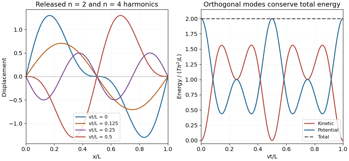
Fixed endpoints select sine normal modes with and . The product identity decomposes the held initial profile into and , with amplitudes and . Zero initial velocity selects cosine time dependence. ThereforeBoth endpoints vanish at every time. At the product-form displacement is recovered and . The implicit leading displacement amplitude is one in the source's chosen length units; including a physical amplitude multiplies the whole solution by .
The total kinetic energy and small-slope elastic potential energy areOrthogonality removes cross terms between the two distinct sine or cosine modes. A mode of amplitude contributes and . For amplitudes and , the prefactors agree. Writing ,Thusindependent of time. This is another instance of equal modal energies for inverse-harmonic string amplitudes. An explicit initial amplitude multiplies every energy by .

For a twice continuously differentiable function, a finite second-order Taylor expansion about an interior point iswhere , , at that point. A differentiable interior extremum requires . For a strict minimum guaranteed by the quadratic term, the Hessian matrix must be positive definite. Completing the square gives . Thus sufficient nondegenerate minimum conditions areIf , the second-order test is inconclusive; for example has a strict minimum at zero despite a zero Hessian. The finite Taylor argument only needs regularity. The source's infinite Taylor representation additionally needs suitable analyticity: a smooth flat function, such as extended by zero at the origin, has every Taylor coefficient zero there but is positive nearby.
At an interior stationary point, let , , and . The quadratic change in the Taylor expansion is negative in every nonzero displacement when the Hessian matrix is negative definite. Applying the minimum test to gives the sufficient nondegenerate maximum conditionsThe quadratic term then dominates the smaller Taylor remainder in a sufficiently small neighborhood, proving a strict local maximum. A vanishing determinant requires higher-order analysis instead.
At an interior stationary point, a negative determinant of the symmetric Hessian matrix means its two eigenvalues have opposite signs. Along their eigenvectors the leading quadratic change has opposite signs, and the higher-order remainder cannot reverse these signs sufficiently close to the point. Hence the nondegenerate saddle condition isWhen the determinant vanishes, a saddle is still possible but is not determined by second derivatives alone: is a simple example. Thus these tests are decisive for nondegenerate stationary points, not an exhaustive classification from first and second derivatives of every smooth function.
The stationarity equations are and . Thus and , so . The real solutions are , and . The Hessian matrix isAt the origin its determinant is , giving a saddle. At either nonzero stationary point it has eigenvalues , so both are strict minima, with value :They are also global minima, because , with equality exactly at those two points. This is the special coefficient choice in a quartic double well with bilinear coupling.
The contours have exchange symmetry and inversion symmetry . Negative levels between and zero form separate loops around the two minima. The zero contour meets itself at the origin, reflecting the saddle there; positive levels form a single outer closed contour. At large radius the positive quartic terms dominate, so the contours remain bounded. There are no contours below .
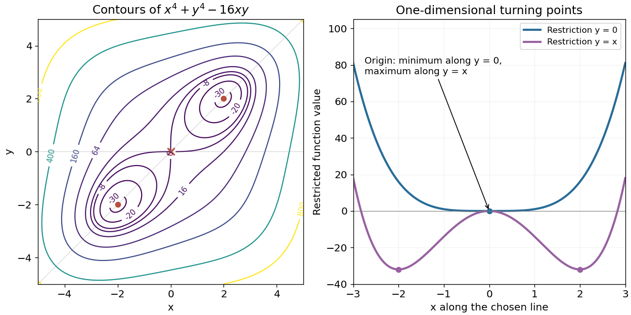
Quartic contours on the required square and one-dimensional restrictions near their turning points
. Details. 
The diagram marks the two minima and central saddle. The restrictions are classified separately below: a minimum or maximum along a single line need not be a two-dimensional extremum.
On , the restricted function is , so changes from negative to positive at zero. HenceThe restricted second derivative vanishes there, but the quartic term determines the minimum. This does not contradict the two-dimensional saddle: values decrease along other directions, including the diagonal near the origin.
On , the restricted function is . Its derivative is , so the turning points are . The restricted second derivative is , negative at zero and positive at . ThusThe corresponding points in the plane are and . Along the diagonal the derivative is , not a single arbitrary partial derivative; here , so their zeros and sign changes agree with the restricted-curve calculation.
Articles by others on the same topic
There are currently no matching articles.