Past exam of the mathematics course of the University of Cambridge / 2001 / ia / Paper 2

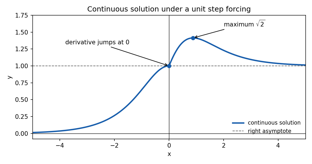
An integrating factor is $\mu (x)=\cosh x$, since ${\mu }^{\prime }/\mu =\tanh x$. ThusFor negative $x$ the integral vanishes; for positive $x$ it is $\sinh x$. ConsequentlyBoth branches give $y(0)=1$. This is Heaviside forcing in a first-order integrating-factor equation: the solution is continuous and piecewise differentiable, while its one-sided derivatives at zero are $0$ and $1$. The Heaviside step function's value at zero does not affect the integral solution. The equation holds classically on the two open half-lines and in the weak sense across zero.

The left branch rises from zero at $-\infty$ to one. On the right,so its unique maximum is $y=\sqrt{2}$ at $x=\mathrm{arsinh}1$, after which it decreases to the horizontal asymptote $y=1$ from above.

The homogeneous characteristic equation is $r^2-r-2=(r-2)(r+1)=0$, so its solutions are $e^{2x}$ and $e^{-x}$. Because the forcing contains the latter exponential, set $y=e^{-x}v$. Direct differentiation reduces the inhomogeneous linear differential equation toA polynomial particular solution is $v=-3x^2-2x$, since $v^{\prime \prime }-3v^{\prime }=-6-3(-6x-2)=18x$. ThereforeThe exponentially growing first term cannot be canceled by the decaying second term, so boundedness at positive infinity requires $C_1=0$. The initial condition $y(0)=1$ sets $C_2=1$. Hence

The side of the inscribed equilateral triangle has length $\sqrt{3}r$. If $d$ is the distance of a chord midpoint from the center, a right triangle gives chord length $2\sqrt{r^2-d^2}$. Thus a chord is sufficiently long exactly when $d<r/2$.

(a) Uniform midpoint area puts the midpoint in the radius-$r/2$ disk with probability(b) Fix the first endpoint by rotational symmetry. Independence and uniformity make the angle $\theta$ of the second endpoint uniform on $[0,2\pi )$. Its chord length is $2r\sin (\theta /2)$, so the required event is $2\pi /3<\theta <4\pi /3$. Hence(c) If the midpoint distance itself has uniform distribution on $[0,r]$, the event $d<r/2$ has probabilityThese are three different probability measures on chords. Their different answers are Bertrand's paradox: specifying what is uniform is indispensable. Uniform area, uniform endpoints and uniform radial distance are not interchangeable sampling rules. Equality at the length threshold has probability zero in all three models.

Use the equally likely release prior, and write $s$ for the probability that the guard names B when A is released. If B is released the guard cannot name B; if C is released the guard must name B. The law of total probability therefore givesA remains jailed and B is named precisely when C is released. Its probability is $1/3$, so the conditional probability isIn (a) unbiased naming has $s=1/2$, giving $2/3$: the guard's claim is false and A's chances have not improved. In (b) preferentially naming B has $s=1$, giving $1/2$: that naming rule makes the claim correct. In (c) preferentially naming C has $s=0$, giving $1$: naming B then reveals that C is the released person, so A certainly remains.

This is the three prisoners problem. The observed name includes information about how the guard selects a name; it is not merely the event that B remains. With general release priors ${\pi }_A,{\pi }_B,{\pi }_C$, the same calculation gives ${\pi }_C/(s{\pi }_A+{\pi }_C)$, making explicit where the equal-prior convention enters.

For the homogeneous linear recurrence relation, substitute $y_k=r^k$. Its characteristic equation of a linear recurrence is $r^2-r+1=0$, with roots $e^{i\pi /3}$ and $e^{-i\pi /3}$. Taking real linear combinations givesThese two real sequences are linearly independent: their values at $k=1,2$ form a matrix with determinant $\sqrt{3}/2\ne 0$. Thus their two constants account uniquely for arbitrary first two values.

Let $P_k={\sum }_{n=1}^k{a}_n/(k-n+1)$ and reindex as $P_k={\sum }_{j=1}^k{a}_{k-j+1}/j$. In $P_{k+2}-P_{k+1}+P_k$, each term with $1\le j\le k$ has coefficientThe term $j=k+1$ is $(a_2-a_1)/(k+1)=0$, and the remaining term is $a_1/(k+2)=1/(k+2)$. This explicitly proves that $P_k$ is the required particular solution, a discrete Green convolution for the period-six recurrence.

The unit-response coefficients have the homogeneous form just found. The values $a_1=a_2=1$ give zero cosine coefficient and sine coefficient $2/\sqrt{3}$, soSubtracting this particular solution from any other solution leaves a homogeneous recurrence. Thus the complete answer is

Where $y_1$ is nonzero, the Wronskian identity $W=y_1{y}_2^{\prime }-y_1^{\prime }{y}_2$ becomes the first-order equationIts integrating factor is $1/y_1$, giving $(y_2/y_1{)}^{\prime }=W/y_1^2$. Integration proves the reduction of order formulaTaking $C_0=0$ gives the displayed representative in the question, with $y_2(x_0)=0$ when $y_1(x_0)\ne 0$. Changing the lower limit adds a multiple of $y_1$ and does not change the linearly independent solution modulo the known one. The scale of $W$ separately fixes the normalization of $y_2$.

Differentiate the determinant and use the original second-order equation for each solution:This proves Abel's identity $W^{\prime }+pW=0$ rather than merely quoting it.

For the specific equation, substituting $y_1=1-x$, $y_1^{\prime }=-1$, $y_1^{\prime \prime }=0$ leaves $(1-x^2)-(1+x)(1-x)=0$. Away from zero its normalized first-derivative coefficient is $p(x)=x-1/x$, soAlthough the equation is singular at zero, this expression extends analytically there. Near zero, $y_1$ is nonzero and the reduction of order integrand is regular. With the prescribed lower limit,The integrand through degree three isAfter integrating and multiplying by $1-x$,The condition $y_2^{\prime \prime }(0)=1$ fixes $C=1$, and the lower limit already gives $y_2(0)=0$. Therefore the first three nonzero terms areThe representation genuinely solves the second-order equation: writing $L[y]=y^{\prime \prime }+p{y}^{\prime }+qy$, differentiating its Wronskian gives $W^{\prime }+pW=y_{1}L[y_2]-y_{2}L[y_1]=y_{1}L[y_2]$. Its left-hand side is zero and $y_1\ne 0$ near zero. Analyticity then extends the original unnormalized equation to zero itself. Its Wronskian with $y_1$ is nonzero for sufficiently small $x\ne 0$, proving linear independence. The vanishing Wronskian at the singular point zero does not contradict linear independence on a regular interval. The integral representation is used locally near zero, before the zero of $y_1$ at one.

Write $A=aI+B$, where $B=\left(\begin{array}{cc}1& -2\\ 1& -1\end{array}\right)$ has $B^2=-I$. One eigenpair isBecause $A$ is real, conjugating $Ae=\ell e$ gives $A\bar{e}=\bar{\ell }\bar{e}$. The eigenvector matrix $(e,\bar{e})$ has determinant $2i\ne 0$, so the eigenvectors form a basis. Reality of $z$ then forces conjugate coefficients, giving $z=\alpha e+\bar{\alpha }\bar{e}$.

Set $c=(1-i)/2$. The forcing has the same basis decomposition,Equating the coefficient of $e$ in the linear system of differential equations yieldsFor $a>0$, an integrating factor gives $\alpha =(c/a)e^{-it}+C{e}^{-(a+i)t}$. The zero initial vector means $\alpha (0)=0$, soTaking the real vector combination givesExact secular resonance occurs at $a=0$: the forcing frequency matches the undamped homogeneous mode. For positive $a$, damping prevents secular growth, and the late-time periodic amplitude is proportional to $1/a$. Thus there is a resonant small-damping limit, but no unbounded resonant response at fixed $a>0$.

Since $(1-e^{-at})/a\to t$ for each fixed $t$, the requested limit givesEquivalently $\alpha =ct{e}^{-it}$ at zero damping; its linear prefactor displays the resonance explicitly.

The term $p$ represents prey reproduction and $-p^2/a$ limits growth by available food, giving carrying capacity $a$ in the absence of hunters. The loss $-ph/a$ represents encounters between prey and hunters. For hunters, $hp/(8b)$ is prey-supported growth and $-h/8$ is mortality; their per-capita growth changes sign at prey population $b$. The coordinate axes are invariant, and positive initial populations remain positive.

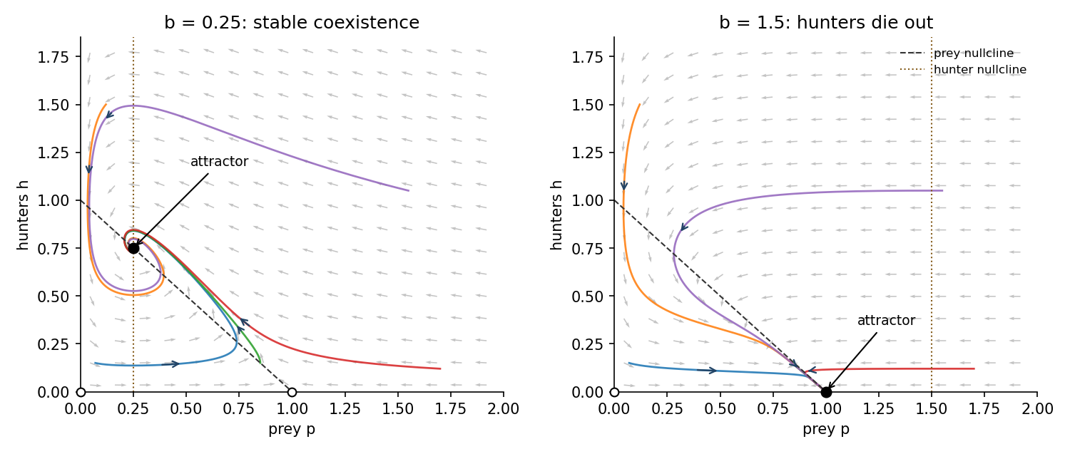
For $a=1$, the physical equilibrium points are the origin, $(1,0)$, and $(b,1-b)$ when $b<1$. The Jacobian matrix isAt $(0,0)$ its eigenvalues are $1$ and $-1/8$, so the origin is always a saddle equilibrium, attracting along the hunter-only axis and repelling along the prey-only axis. At $(1,0)$ the eigenvalues areIt is a saddle equilibrium for $0<b<1/2$ and an asymptotically stable node for $b>1$.

For $0<b<1/2$, the coexistence Jacobian matrix isIts trace is negative and determinant positive. Its discriminant $b^2-(1-b)/2=(2b-1)(b+1)/2$ is negative, so $(b,1-b)$ is an asymptotically stable focus. Interior trajectories approach it in damped, counterclockwise oscillations in the $(p,h)$ plane. Both populations ultimately coexist.

To justify the global interior fate for this logistic predator-prey model, let $h_{\ast }=1-b$ and use the Lyapunov functionIt is nonnegative and its sublevel sets are compact inside the positive quadrant. Differentiation gives the explicit cancellationThe only invariant subset on which this vanishes is $p=b,h=h_{\ast }$: remaining at $p=b$ requires $\dot{p}=b(1-b-h)=0$. LaSalle's invariance principle therefore proves that every strictly positive initial state converges to this coexistence point.

For $b>1$, the formal coexistence point has negative $h$ and is outside the physical state space. The only physical equilibria are the saddle equilibrium at the origin and the stable prey-only node. Since $\dot{p}\le p(1-p)$, positive prey has $\mathrm{limsup}p\le 1$. Eventually $p<b$ with a fixed margin, so hunter population decays exponentially. When $h$ is sufficiently small, comparison with $\dot{p}=p(1-\epsilon -p)$ gives $\mathrm{liminf}p\ge 1-\epsilon$ for every $\epsilon >0$. Thus $h\to 0$ and $p\to 1$ for positive initial prey: hunters die out and prey reaches carrying capacity.

On the boundary, hunter-only initial data approach the origin; prey-only positive data approach $(1,0)$ in either parameter range. The sketches show representative values in the two requested ranges. Dashed and dotted lines are the prey and hunter nullclines; filled dots are attractors and open dots are saddle equilibria.

Let the win probabilities in games 1,2,3 be $u,v,w$. Independence makes a prescribed result pattern the product of its three win/loss probabilities. Taking a complement for event (a), inclusion-exclusion for overlapping pairs in (b) and (c), and disjoint exact-two patterns in (d) and (e), givesFor (b), a three-win outcome is counted three times in the pair sum and must be counted once, so subtract twice its probability. For (c), only the overlapping pairs 12 and 23 are allowed, so subtract the three-win intersection once. For (d), the two allowed exact patterns are 110 and 011. For (e), add 101 as well.

Substituting $(u,v,w)=(q,p,q)$ and $(p,q,p)$ gives the complete comparison:For (a) and (b), the differences $P_{MDM}-P_{DMD}$ are respectively $(p-q)(1-p)(1-q)>0$ and $(p-q)(p+q-2pq)>0$. For (c) and (d), the differences $P_{DMD}-P_{MDM}$ are $pq(p-q)>0$ and $2pq(p-q)>0$. For (e), $P_{MDM}-P_{DMD}=(p-q)(p+q-3pq)>0$ by the additional hypothesis. Thus all maximizing orders follow with strict inequalities.

For a uniform random point in a disk, the event $R<x$ occupies a disk of area $\pi x^2$ when $0<x<1$. ThusThe radial probability density function is $f_R(r)=2r$ on $(0,1)$. Integrating givesChoose the polar angle $\Theta \in [0,2\pi )$. The Cartesian density is $1/\pi$ in the disk, and the polar coordinates Jacobian determinant is $r$. HenceThe product support and product density prove that $R$ and $\Theta$ are independent, with uniform angle.

Reflection symmetry gives $\mathbb{E}X=\mathbb{E}Y=0$ and $\mathbb{E}(XY)=0$, so $\mathrm{Cov}(X,Y)=0$. They are nevertheless not independent. The events $X>3/4$ and $Y>3/4$ each have positive probability, but their intersection is empty inside the disk, because it would require $X^2+Y^2>18/16>1$. Independence would give a positive product probability for that intersection.

Except at the probability-zero center, $X/R=\cos \Theta$ and $Y/R=\sin \Theta$. ThereforeAn arbitrary definition at the center does not change these expected values. This example distinguishes uncorrelated Cartesian coordinates from independent polar coordinates.

A loaded gun remains loaded after its visit with probability $1/2$. An unloaded gun is loaded and then not fired with probability $(3/4)(1/2)=3/8$. The visited gun's new loaded probability is thereforePreservation requires $p^{\prime }=p$, givingThis is product stationarity under single-coordinate Markov updates: the visited coordinate has the same Bernoulli distribution afterward, and its independent local random decisions do not affect the other coordinates. Thus the originally independent indicator random variables remain jointly independent after each scheduled visit, not merely equal in their marginal probabilities.

Let $X_j$ be the indicator random variable that gun $j$ is loaded. Then $N={\sum }_{j=1}^m{X}_j$ has binomial distribution with parameters $m,3/7$. By linearity of expectation and independence of the indicator random variables,

Fix any starting village and let $A$ be the pickup distance, $B$ the subsequent passenger distance. From each vertex, the four possible pickup distances are $0,5,10,15$, each with probability $1/4$. From each pickup village, the three other possible destinations have distances $5,10,15$, each with probability $1/3$.

Sharing the pickup village does not by itself give independence. Here it does hold because the conditional distribution of $B$ is the same for every pickup village: for all allowed $a,b$,Thus $D=A+B$ has the taxi distance convolution on a rectangular road cycle. Counting the twelve equally likely pairs givesNo other distances are possible. The probability distribution is the same for every starting village, so no assumption about the previous customer's destination is needed.

The separate moments are $\mathbb{E}A=15/2$, $\mathbb{E}B=10$, $\mathrm{Var}A=125/4$ and $\mathrm{Var}B=50/3$. Independence therefore givesAs a check from the displayed probability mass function, $\mathbb{E}{D}^2=2125/6$ and subtracting $(35/2{)}^2$ gives the same variance.