Using the Levi-Civita symbol and the contraction of two Levi-Civita symbols, the th component of the vector triple product isThus the triple-product identity is .
Apply this with the unit vector to obtain . Dot products and scalar multiplication are linear in , so . Its matrix representation isThe fixed-vector equation is equivalent to . Since , all its solutions are . Also . Every vector decomposes as , with orthogonal to . Hence is the orthogonal projection onto the plane through the origin normal to : it fixes that plane and removes the perpendicular component.
A family is linearly independent if forces . For the three specified vectors, direct substitution givesThe coefficients are not all zero, so the vectors are linearly dependent.
For the implication question, using the usual interpretation that a basis contains the listed family as independent entries, the answers in order (i)–(x) areThe key distinctions are that the unrestricted zero combination always exists, whereas linear dependence requires a nontrivial combination; and dependence does not necessarily let the specified third vector be solved in terms of the first two. For example , makes (iii) and (iv) false, while disproves (vi).
There is a set-versus-family qualification in (v). If “contains” is interpreted as literal set containment, repeated nonzero vectors need only occur once in the basis. Then is dependent as a family but all three belong to the basis , so (v) becomes false. With three distinct vectors, or with family-containment as above, basis extension gives (v) true. Implication (x) remains true on either reading.
The definition of a convergent sequence isTo prove the product rule, convergence first gives an eventual bound . ThenChoose sufficiently large that and , as well as the bound on . The right side is less than , proving directly from the limit of a sequence definition.
If , eventually , so the reverse triangle inequality gives . ConsequentlyThus . The condition ensures the reciprocal sequence is defined at every index; the nonzero limit supplies the eventual uniform bound away from zero. Finally has every term nonzero, showing that this termwise property alone does not prevent a zero limit.
Suppose is continuous on , differentiable on and satisfies , with . Apply the extreme value theorem to both and to obtain a maximum and a minimum. If is constant, every interior derivative is zero. Otherwise some value differs from the common endpoint value, so either a maximum or a minimum occurs at an interior point . At an interior maximum, difference quotients are nonpositive from the right and nonnegative from the left; since the derivative exists, it must be zero. The minimum case is identical with the inequalities reversed. This proves Rolle's theorem: for some .
For the mean value theorem, subtract the endpoint chord:Then , so Rolle's theorem supplies with . HenceIf everywhere, applying the mean value theorem to any gives . Thus is strictly increasing. The converse is false: is strictly increasing but .
To find the kernel of a linear map, perform the row operations and , followed by . The equivalent homogeneous equations areThe resulting determinant is . If all coordinates vanish. At only remains; at the equations give , . Therefore kernel bases areThe empty family is the basis of the zero vector subspace.
For the change of basis, let be the matrices whose columns are the two ordered bases in standard coordinates. Then , so with . If and represent the same linear map in the two bases, and also . Therefore , andFor the concrete bases, their vectors satisfy , , . These coordinate columns giveAt , every row of is , so every row of is . Multiplying on the left by the displayed inverse givesThe original PDF asks for this full product; its final factor is missing from the converted TeX.
If , then is equivalent to . Thus the solution set is the affine solution space of a linear equation , and every vector of that form solves the equation.
For the symmetric matrix case, let . Symmetry givesDistinct eigenvalues therefore imply . Normalizing the three vectors gives an orthonormal basis. Expand and , with . The equation becomes for every . Thus solvability is equivalent to , and all solutions areThis proves the claimed orthogonality condition and the full solution family rather than only a particular solution.
For the numerical symmetric matrix, direct multiplication gives for , and for . Their orthogonal complement is spanned by , and multiplication gives . The supplied right side has , so the linear system is solvable. Its other coefficients are and . HenceEquivalently, all solutions are
Complete the square in the real-valued complex plane equation:Dividing by gives center and radiusIf the radicand is zero, the locus is the single point , a degenerate circle. If it is negative, the locus is empty. The absolute value of is essential even when .
For the requested sketch, the five centers and radii are respectively , , , and , all centers on the real axis.
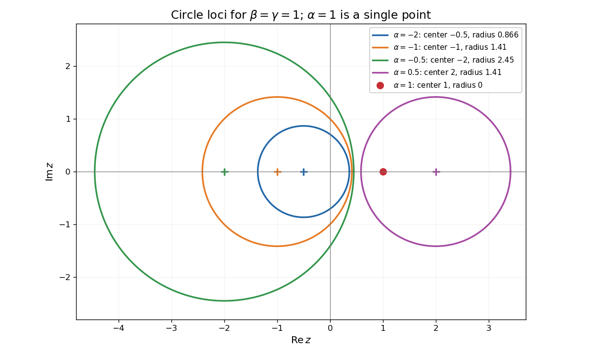
The original PDF's map is ; the converted TeX drops the conjugate on its denominator. Write , so . This is the reflection symmetry of a complex circle equation. It fixes and satisfiesThus it maps every point of the circle into the same circle. Conversely, for any point on that circle, also lies on it and . This proves , including the surjectivity required by the question.
For any three nonempty circles, fix . The triangle inequality gives, for every ,Taking the maximum over proves the requested inequality.
For centers and radii , the maximum separation of two circles is bounded above by . If the centers differ, choose and , where , to attain the bound. If the centers coincide, any unit gives opposite points attaining . ThereforeThe function is not a metric on positive-radius circles, since , even though it satisfies this triangle-type inequality.
The line through the origin is , containing zero and closed under addition and scalar multiplication, so it is a vector subspace. If , then and for some real . Conversely that equality gives the same set after shifting the line parameter. ThusChanging representatives to , changes their sum by and a scalar multiple by . The line classes therefore do not change, proving both operations well-defined. Associativity follows from . The zero vector of this quotient vector space is the entire line , because .
For a basis of , every vector is , so . If this combination equals , then ; independence of the three original basis vectors forces . Hence is a basis of the space of parallel lines as a quotient vector space.
For the specified direction, add to to obtain the representative . Thus its coordinates in the two standard line classes are . The two supplied image classes have coordinates and , while their input coordinates are and . If are the matrix columns, then and . Solving gives
Let bound all and put . ThenThe geometric series converges, so the comparison test for series proves absolute convergence of . This is the bounded power-series terms force interior absolute convergence principle.
Define the radius of convergence byallowing and . If , the supremum supplies a point of convergence with ; convergence makes its terms bounded, so the argument above gives absolute convergence at . If , convergence is impossible by definition. At , no general conclusion follows. Thus the convergence region has a circular interior centered at zero, with boundary behavior depending on the power series.
For ,If , choose strictly between that limit and . Eventually , proving absolute convergence by the geometric series comparison. If , choose below the limit; eventually , so the terms do not tend to zero and the series diverges. The point is harmless. This proves the root test in the needed case and gives
All three examples below have radius of convergence one, because the th roots of their coefficient moduli tend to one.
For convergence everywhere on the boundary, take . On it converges absolutely: for , , whose sum telescopes to a finite value.
For divergence everywhere on the boundary, take . If , every term has modulus one, so the term test for divergence applies.
For mixed boundary behavior, take . At it is the divergent harmonic series; each successive dyadic block contributes at least . At every other point , summation by parts proves convergence. Indeed put , so the finite geometric series gives . ThenThus the partial sums form a Cauchy sequence and converge. This derives the relevant Dirichlet test rather than only naming it.
To prove the intermediate value theorem in this setting, let and . The endpoint inequalities and continuity give an interval immediately to the right of contained in and an interval immediately to the left of disjoint from . Thus . Choose points of tending to ; continuity gives . If , continuity would place some point larger than in , contradicting the supremum. Hence at an interior point.
For a continuous self-map of , define . The range condition implies and . If either is zero, its endpoint is a fixed point. Otherwise apply the just-proved intermediate value theorem to with target zero to obtain and . ThereforeThis proves the fixed-point property of a closed interval without requiring itself to be monotone.
The fixed-point property fails on an open interval. The continuous functionmaps into itself, because . Its only possible fixed point satisfies , hence , which is outside the domain. It is therefore a counterexample even with the self-map requirement retained.
The fixed-point property also fails on the real line. The continuous function maps into itself but has no fixed point, since is impossible.
By continuity of at , for any choose such that whenever . Twice using the fundamental theorem of calculus gives the remainder asThe inner difference is and has modulus at most . Integrating this bound over the interval between and proves, for either sign of ,This is the local quadratic Taylor remainder estimate. The given may enter the bound on the second derivative; no stronger differentiability assumption is needed.
The intermediate value theorem gives a root , unique because makes strictly increasing. We show that Newton root-finding iteration, started at , always stays to the right of . If , the mean value theorem gives for some . Since , is strictly increasing, so . It follows thatInduction gives , so the bounded monotone sequence theorem supplies a limit . The continuous positive is bounded away from zero on , making continuous. Passing to the limit in gives and hence . Uniqueness implies .
For the rate, apply the Taylor theorem with Lagrange remainder to between and :With , rearrangement givesThus the monotone Newton convergence for a strictly convex function has quadratic convergence. More concretely, if , then . Once , induction gives , exhibiting the repeated squaring of small errors.
For a bounded function on a nondegenerate compact interval , a partition has Darboux sumsThe Riemann integrability criterion isEquivalently the supremum of lower sums and infimum of upper sums agree; their common value is the Riemann integral. A bounded nonintegrable example is the Dirichlet function . Every positive-length interval contains rational and irrational points, so every lower sum is zero and every upper sum is .
Suppose the continuous nonnegative function has somewhere. Continuity supplies a positive-length interval within on which ; at an endpoint use a one-sided interval. By monotonicity of the Riemann integral, its contribution to the integral is strictly positive, a contradiction. Therefore under the stated continuous-function assumptions.
For the general integrable case, choose and let while for . This nonnegative indicator function is Riemann integrable with integral zero: isolate in partition intervals of arbitrarily small total length, making the upper sum arbitrarily small while the lower sum stays zero. Yet . This is the single-point changes preserve Riemann integrals phenomenon and supplies the counterexample.
Put . At an interior point and for small enough,By continuity at , the modulus is bounded by the supremum of between and , which tends to zero. Thus the fundamental theorem of calculus givesAt the interval endpoints the same argument supplies the corresponding one-sided derivatives.
For an integrable discontinuous function, the single-point spike from part (i) has , so ; this disproves the derivative identity even when the primitive is differentiable. To see that differentiability itself may fail, take the step function for and for . It is Riemann integrable, but its primitive is and has left derivative zero and right derivative one at . Hence the full assertion is false for general Riemann-integrable functions.
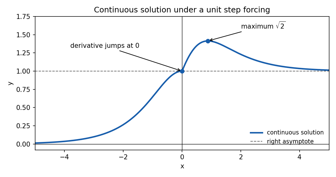
An integrating factor is , since . ThusFor negative the integral vanishes; for positive it is . ConsequentlyBoth branches give . This is Heaviside forcing in a first-order integrating-factor equation: the solution is continuous and piecewise differentiable, while its one-sided derivatives at zero are and . The Heaviside step function's value at zero does not affect the integral solution. The equation holds classically on the two open half-lines and in the weak sense across zero.
The left branch rises from zero at to one. On the right,so its unique maximum is at , after which it decreases to the horizontal asymptote from above.
The homogeneous characteristic equation is , so its solutions are and . Because the forcing contains the latter exponential, set . Direct differentiation reduces the inhomogeneous linear differential equation toA polynomial particular solution is , since . ThereforeThe exponentially growing first term cannot be canceled by the decaying second term, so boundedness at positive infinity requires . The initial condition sets . Hence
The side of the inscribed equilateral triangle has length . If is the distance of a chord midpoint from the center, a right triangle gives chord length . Thus a chord is sufficiently long exactly when .
(a) Uniform midpoint area puts the midpoint in the radius- disk with probability(b) Fix the first endpoint by rotational symmetry. Independence and uniformity make the angle of the second endpoint uniform on . Its chord length is , so the required event is . Hence(c) If the midpoint distance itself has uniform distribution on , the event has probabilityThese are three different probability measures on chords. Their different answers are Bertrand's paradox: specifying what is uniform is indispensable. Uniform area, uniform endpoints and uniform radial distance are not interchangeable sampling rules. Equality at the length threshold has probability zero in all three models.
Use the equally likely release prior, and write for the probability that the guard names B when A is released. If B is released the guard cannot name B; if C is released the guard must name B. The law of total probability therefore givesA remains jailed and B is named precisely when C is released. Its probability is , so the conditional probability isIn (a) unbiased naming has , giving : the guard's claim is false and A's chances have not improved. In (b) preferentially naming B has , giving : that naming rule makes the claim correct. In (c) preferentially naming C has , giving : naming B then reveals that C is the released person, so A certainly remains.
This is the three prisoners problem. The observed name includes information about how the guard selects a name; it is not merely the event that B remains. With general release priors , the same calculation gives , making explicit where the equal-prior convention enters.
For the homogeneous linear recurrence relation, substitute . Its characteristic equation of a linear recurrence is , with roots and . Taking real linear combinations givesThese two real sequences are linearly independent: their values at form a matrix with determinant . Thus their two constants account uniquely for arbitrary first two values.
Let and reindex as . In , each term with has coefficientThe term is , and the remaining term is . This explicitly proves that is the required particular solution, a discrete Green convolution for the period-six recurrence.
The unit-response coefficients have the homogeneous form just found. The values give zero cosine coefficient and sine coefficient , soSubtracting this particular solution from any other solution leaves a homogeneous recurrence. Thus the complete answer is
Where is nonzero, the Wronskian identity becomes the first-order equationIts integrating factor is , giving . Integration proves the reduction of order formulaTaking gives the displayed representative in the question, with when . Changing the lower limit adds a multiple of and does not change the linearly independent solution modulo the known one. The scale of separately fixes the normalization of .
Differentiate the determinant and use the original second-order equation for each solution:This proves Abel's identity rather than merely quoting it.
For the specific equation, substituting , , leaves . Away from zero its normalized first-derivative coefficient is , soAlthough the equation is singular at zero, this expression extends analytically there. Near zero, is nonzero and the reduction of order integrand is regular. With the prescribed lower limit,The integrand through degree three isAfter integrating and multiplying by ,The condition fixes , and the lower limit already gives . Therefore the first three nonzero terms areThe representation genuinely solves the second-order equation: writing , differentiating its Wronskian gives . Its left-hand side is zero and near zero. Analyticity then extends the original unnormalized equation to zero itself. Its Wronskian with is nonzero for sufficiently small , proving linear independence. The vanishing Wronskian at the singular point zero does not contradict linear independence on a regular interval. The integral representation is used locally near zero, before the zero of at one.
Write , where has . One eigenpair isBecause is real, conjugating gives . The eigenvector matrix has determinant , so the eigenvectors form a basis. Reality of then forces conjugate coefficients, giving .
Set . The forcing has the same basis decomposition,Equating the coefficient of in the linear system of differential equations yieldsFor , an integrating factor gives . The zero initial vector means , soTaking the real vector combination givesExact secular resonance occurs at : the forcing frequency matches the undamped homogeneous mode. For positive , damping prevents secular growth, and the late-time periodic amplitude is proportional to . Thus there is a resonant small-damping limit, but no unbounded resonant response at fixed .
Since for each fixed , the requested limit givesEquivalently at zero damping; its linear prefactor displays the resonance explicitly.
The term represents prey reproduction and limits growth by available food, giving carrying capacity in the absence of hunters. The loss represents encounters between prey and hunters. For hunters, is prey-supported growth and is mortality; their per-capita growth changes sign at prey population . The coordinate axes are invariant, and positive initial populations remain positive.
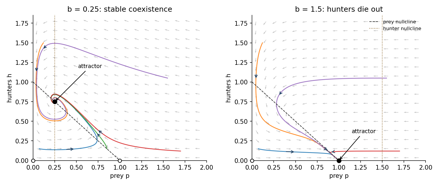
For , the physical equilibrium points are the origin, , and when . The Jacobian matrix isAt its eigenvalues are and , so the origin is always a saddle equilibrium, attracting along the hunter-only axis and repelling along the prey-only axis. At the eigenvalues areIt is a saddle equilibrium for and an asymptotically stable node for .
For , the coexistence Jacobian matrix isIts trace is negative and determinant positive. Its discriminant is negative, so is an asymptotically stable focus. Interior trajectories approach it in damped, counterclockwise oscillations in the plane. Both populations ultimately coexist.
To justify the global interior fate for this logistic predator-prey model, let and use the Lyapunov functionIt is nonnegative and its sublevel sets are compact inside the positive quadrant. Differentiation gives the explicit cancellationThe only invariant subset on which this vanishes is : remaining at requires . LaSalle's invariance principle therefore proves that every strictly positive initial state converges to this coexistence point.
For , the formal coexistence point has negative and is outside the physical state space. The only physical equilibria are the saddle equilibrium at the origin and the stable prey-only node. Since , positive prey has . Eventually with a fixed margin, so hunter population decays exponentially. When is sufficiently small, comparison with gives for every . Thus and for positive initial prey: hunters die out and prey reaches carrying capacity.
On the boundary, hunter-only initial data approach the origin; prey-only positive data approach in either parameter range. The sketches show representative values in the two requested ranges. Dashed and dotted lines are the prey and hunter nullclines; filled dots are attractors and open dots are saddle equilibria.


Let the win probabilities in games 1,2,3 be . Independence makes a prescribed result pattern the product of its three win/loss probabilities. Taking a complement for event (a), inclusion-exclusion for overlapping pairs in (b) and (c), and disjoint exact-two patterns in (d) and (e), givesFor (b), a three-win outcome is counted three times in the pair sum and must be counted once, so subtract twice its probability. For (c), only the overlapping pairs 12 and 23 are allowed, so subtract the three-win intersection once. For (d), the two allowed exact patterns are 110 and 011. For (e), add 101 as well.
Substituting and gives the complete comparison:For (a) and (b), the differences are respectively and . For (c) and (d), the differences are and . For (e), by the additional hypothesis. Thus all maximizing orders follow with strict inequalities.
For a uniform random point in a disk, the event occupies a disk of area when . ThusThe radial probability density function is on . Integrating givesChoose the polar angle . The Cartesian density is in the disk, and the polar coordinates Jacobian determinant is . HenceThe product support and product density prove that and are independent, with uniform angle.
Reflection symmetry gives and , so . They are nevertheless not independent. The events and each have positive probability, but their intersection is empty inside the disk, because it would require . Independence would give a positive product probability for that intersection.
Except at the probability-zero center, and . ThereforeAn arbitrary definition at the center does not change these expected values. This example distinguishes uncorrelated Cartesian coordinates from independent polar coordinates.
A loaded gun remains loaded after its visit with probability . An unloaded gun is loaded and then not fired with probability . The visited gun's new loaded probability is thereforePreservation requires , givingThis is product stationarity under single-coordinate Markov updates: the visited coordinate has the same Bernoulli distribution afterward, and its independent local random decisions do not affect the other coordinates. Thus the originally independent indicator random variables remain jointly independent after each scheduled visit, not merely equal in their marginal probabilities.
Let be the indicator random variable that gun is loaded. Then has binomial distribution with parameters . By linearity of expectation and independence of the indicator random variables,
Fix any starting village and let be the pickup distance, the subsequent passenger distance. From each vertex, the four possible pickup distances are , each with probability . From each pickup village, the three other possible destinations have distances , each with probability .
Sharing the pickup village does not by itself give independence. Here it does hold because the conditional distribution of is the same for every pickup village: for all allowed ,Thus has the taxi distance convolution on a rectangular road cycle. Counting the twelve equally likely pairs givesNo other distances are possible. The probability distribution is the same for every starting village, so no assumption about the previous customer's destination is needed.
The separate moments are , , and . Independence therefore givesAs a check from the displayed probability mass function, and subtracting gives the same variance.
Put and . Direct matrix multiplication gives the two-dimensional Cayley-Hamilton theorem identity . If , determinant multiplicativity gives , hence . The identity then says . If , its trace is zero; otherwise a nonzero entry forces . Thus and .
Conversely, those two scalar relations give , so the same Cayley-Hamilton theorem identity implies . ThereforeThis is the square-zero criterion for a two-by-two matrix. If , determinant multiplicativity first gives , hence . Now and . Either , or a nonzero entry gives and hence ; in both cases . The converse follows by multiplying by . Consequently . A nonzero nilpotent matrix of this size therefore has nilpotency index two.
A Möbius transformation is with . On the Riemann sphere, a zero denominator represents infinity, and when ; when , infinity is fixed. The numerator and denominator cannot vanish together because .
The matrix acts on homogeneous coordinates , so composition satisfies . The product is invertible since , proving closure. Composition is associative because these are maps of the sphere. The identity is , andis again a Möbius transformation. Thus the transformations form a group. Nonzero scalar multiples of a matrix give the same transformation, but the identity and inverse assertions concern the transformations themselves.
Write , with , and . If , then and . If , division givesHence the Möbius translation-scaling-inversion factorization isThe scaling coefficient is nonzero. At the reciprocal sends the translated zero to infinity; at infinity it sends infinity to zero. Thus the factorization holds on the entire Riemann sphere, including both exceptional points, and proves the stated generating property.
For a differentiable scalar function and a differentiable curve, the multivariable chain rule isLet . Choose to be an invariant of the method of characteristics. Then , so and a convenient choice is . For , the chain rule gives . Thus, writing the unknown in the new coordinates,Integrating with fixed yieldswhere is an arbitrary differentiable function on the relevant interval. This gives all local solutions on each patch where the specified change of variables is invertible: its Jacobian determinant is .
The axes need care because is undefined at and the Jacobian vanishes at . Reparameterizing gives the simpler chart expressionIt is the general solution on either component or , including when is differentiable there. Indeed is a nonsingular coordinate chart for , and the weighted Euler first-order equation reduces to .
For a patch crossing with , the characteristic invariant instead gives , with an arbitrary differentiable function on each sign component of . These chart descriptions must agree on overlaps. On the axes the original equation gives and on their separate components; a solution defined smoothly through the origin must have and compatible smooth limits, in particular . No boundary data select a particular arbitrary function.
Consider the globally smooth potential . Direct differentiation givesThus the differential one-form is the exact differential , proving exactness rather than only checking a necessary condition on its partial derivatives. Along any piecewise differentiable path, the chain rule gives . The fundamental theorem of calculus therefore makes the line integral depend only on its endpoints:
An eigenvalue of is a scalar for which a nonzero vector satisfies . Equivalently, , because the homogeneous linear system has a nontrivial solution exactly when its coefficient matrix is singular. This characteristic polynomial is the monic quadraticA nonzero quadratic has at most two distinct roots, proving the eigenvalue bound. Eigenvalues and diagonalization are taken over , also for a matrix with real entries.
For the matrix commutator, the cyclic trace identity follows directly from its entries:Hence . Factoring the characteristic polynomial as and comparing the coefficient of gives , with the eigenvalues counted with algebraic multiplicity. If both eigenvalues are zero, trace and determinant are zero. The Cayley-Hamilton theorem then gives ; no diagonalizability assumption is needed.
Now put . Since its trace is zero, its characteristic polynomial is and the scalar square of a traceless two-by-two matrix identity givesThis proves the scalar-square assertion for both real and complex entries. If , it gives . If , the two eigenvalues are the distinct nonzero numbers . Their eigenvectors are linearly independent: a nonzero vector cannot satisfy two different eigenvalue equations. They form a basis, making a diagonalizable matrix. Thus either the commutator is diagonalizable over or its square is zero. These alternatives need not be disjoint, since the zero matrix has both properties. Over the diagonalization assertion would require real eigenvalues; complex diagonalization is essential to the unrestricted statement.
A left group action of on a set is a map satisfying and . The group orbit of is , and its stabilizer subgroup is . The stabilizer subgroup contains the identity, is closed under products, and contains whenever it contains , so it is indeed a subgroup.
The orbit-stabilizer theorem for a finite group saysTo prove it, map a left coset to . This is well-defined because every element of fixes . Conversely, precisely when , which is precisely equality of the two cosets. Thus this map is a bijection between the cosets and the group orbit. Each coset has elements, by the bijection , and the cosets partition , giving the formula.
Apply this to the rotational symmetry group of a cube acting on its six faces. The action is transitive: rotations through right angles about coordinate axes can send the top face to each of the other faces. A rotation fixing a face must fix its outward normal, so it rotates about the axis through that face's center and the opposite face's center. Preservation of its square boundary permits exactly four angles modulo : . All four preserve the cube, so this face stabilizer subgroup has order four. The group is finite because a rotation permutes the six face normals and is determined by their images. The orbit-stabilizer theorem givesThese are orientation-preserving rotations; reflections are not being counted.
Lagrange's theorem states that for a subgroup of a finite group , ; in particular divides . This follows by partitioning into cosets, each in bijection with .
If is prime, take any . Its cyclic subgroup has order dividing , but its order is not one. Thus it has order and equals . HenceThis describes a single group isomorphism type for each prime.
Now let have order , and let be any subgroup. Choose the least positive integer with ; this exists because , even when is trivial. Divide with . Since , minimality forces , so divides . Likewise, dividing an exponent for any shows . Therefore .
Conversely, for each divisor of , is a subgroup of order . The least positive exponent property makes unique. This proves the complete subgroups and quotients of a cyclic group classification:The choices and include the trivial subgroup and the whole group.
Compose permutations from right to left. The indicated cycle lengths immediately give . Under conjugation, . Since sends to and fixes ,Direct composition also gives . Thus is a Klein four-group. Conjugation by cycles its three nonidentity elements, so normalizes .
The cosets have four elements each and are distinct. If two coincided, a nontrivial power of would belong to , impossible because it has order three whereas every nonidentity element of has order two. Hence the subgroup generated by contains at least twelve elements. These generators are even permutations, so the subgroup lies in the alternating group , whose order is ; multiplying by one fixed transposition pairs even and odd permutations to justify this count. ThereforeThe calculation also describes as the semidirect product , with the order-three factor permuting the three involutions.
The direct product of groups uses componentwise multiplication:Associativity follows in each factor. The maps and are injective group homomorphisms onto subgroups, giving the required copies of and .
Use the PDF's convention that the subscript in is the group order. Write the hexagon group as and the triangle group as . Let generate . In , has order three and conjugates it to its inverse, so is a copy of . The element has order two and is central, since .
DefineThe generator relations are preserved and commutes with the other images, so is a group homomorphism from the direct product. The six residues are distinct modulo six: reduction modulo two first determines , then reduction modulo three determines . Together with , they give all twelve distinct normal forms in . Thus is bijective andThis is the dihedral splitting when the half-rotation order is odd with half-rotation order three.
Finally, contains an element of order six, namely . The even cycle types on four symbols are the identity, a 3-cycle, and two disjoint transpositions; their orders are respectively one, three and two. Therefore has no element of order six. Since a group isomorphism preserves element orders,
At a critical point of a twice continuously differentiable real function, the Taylor expansion isThe Hessian matrix is real symmetric, so an orthogonal eigenbasis diagonalizes its quadratic form. If every eigenvalue is positive, that form is bounded below by a positive multiple of , which dominates the remainder and gives a strict local minimum. If every eigenvalue is negative, the same argument gives a strict local maximum. If both signs occur, displacement along the corresponding eigenvectors produces values above and below , so the point is a saddle point of a scalar function. These exhaust a nonsingular Hessian matrix.
A singular Hessian matrix does not always make the classification impossible: nonzero eigenvalues of both signs still give a saddle. If the Hessian matrix is positive or negative semidefinite, higher-order terms in its null directions must be examined. For example, and have the same Hessian matrix at zero, but the first has a strict minimum and the second a saddle. The function has a non-strict minimum along a whole line.
For the given polynomial,A stationary point has and then . Hence the origin is always critical, and two additional points exist exactly for :The Hessian matrix isAt the origin it is , giving a strict local minimum for and a saddle for . At either extra critical point it has determinant , so both extra points are saddles.
At , complete the square:Along it is positive away from zero, whereas along it is negative away from zero. Thus the origin remains a degenerate saddle despite its nonnegative Hessian matrix. This is the parabolic quartic critical-point classification. The complete result isFor the local minimum is not global, since along the same parabola .
For a one-to-one continuously differentiable change of variables with nonzero Jacobian determinant, the change of variables formula rule iswhere is the transformed region and the inverse map covers once. The absolute value is required even if the coordinate map reverses orientation.
Here are positive. For , , the inverse is and . On the first portion of , the bounds give , and because . Together these give ; conversely these inequalities imply and the original bounds. On the second portion, they give , and , hence , with the converse following similarly. The two triangles combine into the rectangle , sharing only the diagonal corresponding to .
The divergence theorem states that a continuously differentiable vector field on a bounded region satisfieswith outward unit normal and a sufficiently regular boundary; piecewise smooth boundaries are also allowed. For with constant , the left side is and the right side is . Equality for every constant vector gives the gradient volume-to-boundary identityFor the cone and its cap, the volume has and in cylindrical coordinates. Its volume is . Since ,The cap at has area , outward normal and , so its contribution to the surface integral is .
Parameterize the side by , , . The outward vector area element ispointing radially outward and downward from the region above the cone. The radial part integrates to zero around the circle. The vertical part of the side integral isAdding cap and side givesThe apex and circular rim have zero surface area. Alternatively, removing a tiny apex neighborhood and taking its radius to zero justifies applying the smooth-boundary theorem there; the additional flux vanishes because the scalar field is bounded.
Let be two sufficiently regular solutions with the same source and boundary data, and set . Then and . Green's first identity givesThe left side is nonnegative, so it vanishes. Thus is constant on each connected component. Its normal derivative is zero, and the boundary condition then forces that constant to be zero. This proves at most one solution. The Poisson uniqueness with a nonnegative Robin normal coefficient proof never divides by , so it includes the points or boundary portions where .
For the exponential-sine modes, direct differentiation givesTheir sum is zero, so both modes are harmonic functions for every real .
For the square, the horizontal Dirichlet data suggest separation of variables in the form , where the positive integer makes the sine vanish at both horizontal edges. The Laplace equation gives , hence . At , the outward normal points in the negative direction. The Robin boundary condition is therefore , or . The right edge requires , fixing the remaining coefficient. The resulting separated Laplace mode with a Robin edge isThe denominator is positive for . The function satisfies the Laplace equation and all four boundary conditions directly; for example its left-edge value and derivative agree, giving the correct outward-normal Robin sign. It extends regularly to the corners.
On the left edge the uniqueness coefficient is ; on the other three edges it is with the prescribed Dirichlet value. The same Green's first identity argument applies to the square's piecewise smooth boundary, whose corners have zero boundary measure. Thus this is the unique regular solution, or equivalently the unique finite-energy solution with these boundary traces. Unbounded corner singularities are outside that boundary-value class.
Suppose were a surjection onto the power set of the set . Form the subsetSurjectivity would give with . But then holds exactly when , a contradiction. Hence no such surjection exists, and in particular there is no bijection between a set and its power set. This is the diagonal construction in Cantor's theorem; it also covers the empty set, whose power set has one element.
No such set exists. If had precisely the sets satisfying as its elements, applying that membership criterion to itself would givea contradiction. This is Russell's paradox. It rules out this unrestricted universal collection; a set whose elements happen not to contain themselves is perfectly possible, for example the empty set.
Articles were limited to the first 100 out of 130 total.
Articles by others on the same topic
There are currently no matching articles.