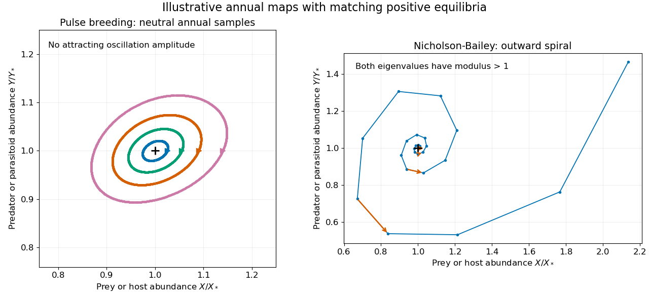
The payoff-table area for Question 6 on page 3 is blank in the Part III PDF and PostScript edition, and in the MPhil PDF and MPhil PostScript edition. All four copies have been checked visually. The solution therefore keeps the payoffs symbolic.
Let be prey and predator abundances. With constant positive demographic and predation coefficients, the Lotka-Volterra equations areTheir positive equilibrium is , . Its Jacobian matrix and eigenvalues areThe linearized populations oscillate with period , with the predator peak following the prey peak. This is a center equilibrium, not an attracting equilibrium. The conclusion is supported beyond linearization by the Logarithmic first integral of the Lotka-Volterra equations: in these units one may useDirect differentiation gives . Its Hessian matrix is a positive-definite matrix in the positive quadrant, and its minimum is at . Nearby level curves are closed periodic orbits, so there is no damping toward a preferred oscillation amplitude.
Use an annual pulse-breeding predator-prey model. Let be the abundances just after reproduction, and let the year have length . Between breeding pulses, assume mass-action predation, natural mortality rates , and no reproduction:Solving the predator equation and inserting it into the prey equation gives the pre-breeding abundancesSuppose reproduction multiplies surviving prey by and adds offspring per surviving predator. Retaining the surviving adults gives , . Define , , and . The resulting difference equations areThus offspring depend on prey available at the end of the year, not on the number killed during the year. The adult-survival convention is part of the model; if breeding replaces all adults, use instead. Both are consistent pulse models under their respective life-history assumptions.
For the adult-survival annual pulse-breeding predator-prey model, a positive annual fixed point exists when and :At this point the Jacobian matrix isIf , the two eigenvalues are a complex conjugate pair of moduli one. The annual samples show linearly neutral seasonal oscillations. If , they form a reciprocal negative real pair and the fixed point is a saddle fixed point of a map. Equality at four is a degenerate boundary needing nonlinear analysis. For replacement rather than surviving adults the same calculation gives trace and determinant one.
The absence of an attracting annual cycle is stronger than a linear observation. Put , . The update becomesIt is the composition of two nonlinear shear maps, each of determinant one: an area-preserving seasonal predator-prey map. No isolated positive periodic orbit has an open attracting basin. Neutral linear oscillations alone also do not prove nonlinear stability at every resonance. In particular, this density-independent model does not select an asymptotically stable oscillation amplitude.
The Nicholson-Bailey model instead counts parasitoid offspring from attacked hosts:Its positive equilibrium has and . Its Jacobian matrix hasSince the determinant exceeds one while the positive trace is below two, the eigenvalues are complex with moduli greater than one: instability of the Nicholson-Bailey equilibrium produces outward oscillations near it. The two maps share an exponential prey-survival factor but have different reproduction laws and stability properties.

Let measure the relative trapping vulnerability and use fixed species-specific catches . With no natural interaction, the two populations satisfy independent constant-quota harvested logistic growth equations,This treats as a common harvest scale: a total fixed quota can equivalently be allocated in fixed fractions . Catches are not reassigned after one species disappears. Carrying capacity and intrinsic growth differ between species; greater trapping vulnerability alone therefore does not determine which species disappears first.
The maximum natural surplus occurs at . Define the critical harvesting levelFor there are two positive equilibria,The derivative of the population vector field is negative at the upper branch and positive at the lower branch. The upper branch is attracting; the lower is an unstable survival threshold. An initial abundance above the lower branch approaches the upper branch, whereas one below it reaches extinction. At , positive populations approach , while zero remains zero.
At the branches meet in a saddle-node bifurcation andInitial abundances above approach it algebraically from above; those below decline to extinction. For there is no positive equilibrium and the derivative of abundance is everywhere negative. In fact , giving finite extinction time. At zero the biological model stops harvesting and keeps the population extinct rather than extending the constant-quota equation to negative abundance.
Order the thresholds as . Below the first threshold, both species can persist if each starts above its own survival threshold; either or both can still disappear from inadequate initial abundance. Between the thresholds only species 2 can persist. Above the second, neither can persist. At each threshold use the one-sided critical behaviour just derived. Equal thresholds give simultaneous loss of both positive branches. Because the equations are independent, there are no sustained oscillations or competitive replacements in this model.
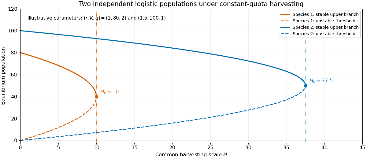
Stable and unstable equilibrium branches of two independently harvested logistic populations
. Details. 
A microparasite typically multiplies within an infected host on a much shorter time scale than between-host transmission. A useful first model classifies hosts by infection status. A macroparasite, such as an adult parasitic worm, instead requires a count of parasites per host: two infected hosts can carry very different within-host parasite burdens. These are modelling distinctions rather than a rule determined only by an organism's physical size.
For a microparasite with no lasting immunity, a homogeneous SIS model isThe basic reproduction number is , and the prevalence describes the infected-host fraction. A SIR model adds an immune class, and a SEIR model adds a latent class. Contact structure, age, susceptibility, recovery rate and infectiousness can require several such classes. Then a next-generation matrix or operator, rather than a single averaged contact rate, sets the invasion threshold. Stochastic epidemic models are relevant to early extinction and finite populations; network or spatial models represent nonuniform contact opportunities.
For a simple macroparasite burden model, let be the fraction of hosts carrying adult worms. Assume acquisitions at rate , independent adult-worm losses at rate , and a number of infective stages in a well-mixed environmental reservoir. The immigration-death worm-burden model hasThis birth-death process needs the burden distribution or its probability generating function, not just an infected/not-infected partition. Its mean satisfies . With host number fixed and each adult producing infective stages at rate , one possible environmental closure isFor this asexual, unsaturated transmission approximation, one worm's basic reproduction number is . Growth above the invasion threshold requires additional density regulation if a finite endemic burden is sought. Sex-dependent mating would change this closure.
With constant external exposure , the equilibrium burden follows a Poisson distribution with mean , giving infected-host prevalence . If exposure rates vary across hosts as a gamma distribution, the Poisson-gamma mixture gives a negative binomial distribution with mean and aggregation parameter :The same mean burden can therefore coexist with very different prevalence and highly infected subgroups. Aggregation of macroparasite burdens affects treatment coverage, burden-dependent host mortality, immunity and parasite fecundity. For sexually reproducing worms, hosts need both sexes for fertile output; a mean alone may not determine it. With independent equally likely sexes and Poisson burden, the probability of both sexes is , illustrating mating-limited macroparasite transmission and its low-burden bottleneck.
Both microparasite and macroparasite models need heterogeneous exposure and host responses. The special extra difficulty for macroparasites is translating a distributed worm burden, and possibly worm sex or developmental stage, into transmission and host harm. Conversely, complicated within-host microparasite processes can also require more than a binary host state when the simple fast-within-host approximation fails.
Let be the infectious proportion in a closed population. With homogeneous frequency-dependent transmission rate and recovery rate , the SIS model isThe basic reproduction number is the expected number of secondary infections produced by a typical newly infected individual in an otherwise susceptible population under the specified contact conditions. Here the infectious duration has mean , so .
For the attracting endemic equilibrium has . The homogeneous SIS susceptible fraction is thereforeFor the physical equilibrium is disease-free, , . At equality approach to zero is algebraic. Thus is an endemic relation, not a formula demanding more than one susceptible person per person below the invasion threshold.
Use an assortatively mixed two-risk-group SIS model with equal per-person recovery rate . Let be infectious proportions in groups of sizes . Let be their fixed contact rates and the transmission probability per contact. Suppose a small fixed fraction of high-risk contacts is with the low-risk group. Contact reciprocity in a two-group epidemic requiresFor sufficiently small , both groups make most contacts within their own group, and the total cross-group contacts are of order . Define , , and . The forces of infection giveHere and hold in the small- regime. High-risk per-person cross contact is order one but its group size is order ; low-risk per-person cross contact is order . These distinctions are needed to count each cross-group partnership consistently.
Linearize about the disease-free state. In infectious fractions the transmission matrix isIn infected-individual counts the next-generation matrix is insteadThe count and fraction formulations are related by a diagonal change of coordinates, so their eigenvalues coincide. The basic reproduction number is the spectral radius , not an average of the two group reproduction numbers. The larger real eigenvalue isThis model makes a particular reciprocal mixing convention explicit; different defensible contact laws can change the first-order coefficients.
The high-contact assumptions give away from a degeneracy. Since , perturbing the larger eigenvalue in the assortatively mixed two-risk-group SIS model givesFor the biologically useful high-risk-core regime , put . Substituting and into the two equilibrium equations givesThus the group susceptible fractions and their population-weighted total areThe small-core SIS endemic expansion shows why the homogeneous SIS susceptible fraction relation fails for a mixed population: as the high-risk fraction tends to zero, while . A small high-risk core sustains infection even though almost everyone in the population remains susceptible. Even need not equal at first order.
For completeness, if with a fixed gap from threshold, small gives disease-free equilibrium and total susceptibility one. If , the low-risk group already sustains infection. Put and let be the positive root of . The first-order coefficients areAgain it tends to rather than . These regular expansions require fixed nonzero gaps. At the spectral splitting is generally order ; at , low-risk infection is also order , so a regular first-order Taylor expansion is inappropriate. An exact endemic replacement for the scalar identity is that the susceptible-weighted next-generation matrix has spectral radius one.
Let be the allele frequency of , with random mating and sufficiently large population size to neglect genetic drift. The Hardy-Weinberg proportions before selection are . Write the three genotype fitnesses as , with smaller than either homozygote value. After one viability-selection generation,ConsequentlyPut , . The underdominant allele-frequency dynamics has stable fixation states zero and one, separated by the unstable thresholdBelow it decreases to allele fixation of ; above it increases to fixation. Exactly at the threshold the deterministic frequency remains balanced, but any perturbation selects a side. This is underdominance, or heterozygote disadvantage, rather than balancing selection from heterozygote advantage.
In a continuous-time weak-selection or selection-rate convention, the corresponding equation is . Equal homozygote fitness gives for a positive selection strength . The next part uses this explicitly stated continuous-time convention; and migration then have the same time units.
Use a globally coupled underdominant metapopulation with equal habitat sizes:Symmetry preserves a common frequency in the initially habitats and in the initially habitats. With , the equations reduce exactly toThe maximum positive selection rate is at . Comparing it with the worst outward migration flux gives a sufficient barrier condition . A slightly stronger optimized condition follows from maximizing the per-capita restoring term over : its maximum is at .
Indeed, on , with , . On , with , . The other two edges point inward as well. The invariant-rectangle criterion for underdominant coexistence therefore gives the explicit robust conditionsStarting from the specified pure habitats, the populations then remain in , . Their global frequency lies between and , so neither allele fixes. This is a sufficient condition, not a claim that the bound is sharp. If or , the population is already fixed; if , any mixture of the two pure habitat types persists.
The exactly balanced case illustrates why robustness and the prescribed trajectory differ. When , symmetry forces andFor its heterogeneous limiting state isHere , so the full Jacobian matrix has diagonal entries and off-diagonal entries . Its two full-system eigenvalues are and : the symmetric underdominant two-cluster equilibrium is robustly attracting only for . For larger migration the exactly symmetric initial condition can still avoid fixation, eventually approaching the spatially uniform frequency when , but the symmetry-broken mean-frequency mode is unstable. A finite population with genetic drift need not maintain deterministic coexistence indefinitely.
The payoff table is blank in the original PDF, so denote its four row-player payoffs by for , with the prisoner's dilemma ordering . No numerical entries are inferred. Let the two reactive strategies be and , where is cooperation after the opponent's cooperation and cooperation after defection.
The joint action states form a four-state Markov chain. In state order , its transition matrix isThe prescribed initial memories give independent first actions with cooperation probabilities . Same-round actions remain independent: each player's next action uses the other player's previous action and its own independent random draw. Thus their marginal cooperation probabilities obeyPut . If , the two-step recurrences contract and the long-run payoff of reactive strategies follows fromThe joint stationary distribution is . Player 1's mean payoff is ; exchange for player 2.
The deterministic boundaries must retain the initial memories rather than divide by zero. Two Tit for tat players cooperate forever and earn . Two players who always do the opposite of the opponent's previous action alternate and average . One of each cycles through all four states and each averages . These are the only cases with . A periodic Markov chain need not have convergent state probabilities, but its long-time average payoff is defined by its cycle frequencies.
Under the standard two-condition criterion for evolutionary stability, the strict claim fails. Tit for tat and always cooperate both cooperate in every round when playing either each other or their own type under the specified initial memories. HenceBoth stability comparisons tie. The neutrality between Tit for tat and unconditional cooperation proves that Tit for tat is not an evolutionarily stable strategy in the stated strategy space, and cannot strictly invade every strategy. The final differently spelled name is interpreted as the same rule, since no second strategy is defined.
There is a useful qualified invasion result. For a resident with , put . The long-run payoff of reactive strategies givesThus, if the fraction of Tit for tat players is , their payoff advantage isMoreover . Under the additional cooperative-efficiency condition , this is positive whenever . Tit for tat invasion of a reactive resident then occurs from every positive frequency, although its invasion exponent at frequency zero vanishes. The replicator equation is , so the initial increase is slow and frequency-dependent. Residents with remain cooperative on all reached histories and tie instead. If , some almost-cooperative residents have , and even this qualified invasion conclusion fails.
For the exceptional opposite-response resident , its self-payoff is while its payoff in either order against Tit for tat is . The advantage is . Under , invasion at arbitrarily small frequency requires ; otherwise it needsFinally, taking an infinite undiscounted average before the rare-mutant limit is essential. In an -round match against always defect, the first round contributes to Tit for tat and to the defector, followed by rounds of payoff . The finite-horizon invasion threshold of Tit for tat against unconditional defection isprovided the denominator is positive and the threshold is below one. Thus a finite horizon generally prevents invasion from an arbitrarily rare introduction. The source's absent payoff table prevents choosing which extra payoff inequalities were intended, but the symbolic cases and the strict-ESS counterexample do not depend on guessing it.
Articles by others on the same topic
There are currently no matching articles.