Past exam of the mathematics course of the University of Cambridge / 2001 / iii / Paper 53 (Renormalisation in Dynamical Systems)

The image of the full interval under the tent map is $T_s([-1,1])=[1-s,1]$. Since $s>1$, this image contains the critical point zero and the right endpoint one; its next image is again $[1-s,1]$. Moreover, any interval $B$ with $T_s(B)=B$ lies inside the image of $[-1,1]$. Thus the core interval of an expanding tent map isEvery point outside $A$ enters $A$ after one iterate and then stays there. For $s=2$ there are no points of the domain outside $A$.

To prove interval exactness of a tent-map core, first take a nondegenerate closed interval $L\subseteq A$ and put $L_n=T_s^n(L)$. Each $L_n$ is an interval. If $L_n$ does not straddle zero, the corresponding branch is affine with slope of magnitude $s$, so $|L_{n+1}|=s|L_n|$. If it straddles zero, its image has right endpoint one andIf both $L_n$ and $L_{n+1}$ contain zero, then $L_{n+1}$ contains $[0,1]$, whence $L_{n+2}=A$. Otherwise at most one of these two steps folds across the critical point. Consequently, unless the full core has already been reached,Since $s^2/2>1$, indefinite failure to reach $A$ would give intervals of unbounded length inside an interval of length $s$. This is impossible, proving $\boxed{T_s^k(L)=A\text{ for some }k}$. For an interval with open endpoints, apply the argument to any nondegenerate closed subinterval inside it; its image already covers $A$, while the image of the original interval cannot leave $A$.

Now let $U$ be any nonempty relatively open subset of $A$ and choose a closed nondegenerate $J=[u,v]\subset U$. Some $F=T_s^k$ maps $J$ onto $A$, so there are points $p,q\in J$ with $F(p)=1-s$ and $F(q)=1$. Therefore $F(p)-p\le 0$ and $F(q)-q\ge 0$. The intermediate value theorem yields $z\in J$ with $F(z)=z$. This is a periodic point of $T_s$, of period dividing $k$. Every such $U$ contains one, so the periodic points are dense in the whole core $A$.

Use the interval exactness of a tent-map core from the preceding part. Choose two separated nondegenerate closed intervals $J_0,J_1$ inside $J=(1-s,1)$. There are integers $n_i$ with $T_s^{n_i}(J_i)=A$. Taking $N=\max (n_0,n_1)$ works for both, because $T_s(A)=A$:Within each $J_i$, the continuous function $F$ attains both endpoint levels $1-s$ and $1$. Choose a segment between those levels, reversing its orientation if necessary. Starting from a point at level $1-s$, take the first point at level one, and then the last point at level $1-s$ before it. Between these two points, continuity and the first-passage choice give $1-s<F(x)<1$, with all intermediate levels attained. The interior $K_i$ of that segment therefore satisfies $F(K_i)=J$. The intervals $K_0,K_1$ are disjoint and lie inside $J$.

Thus interval exactness produces a horseshoe:This is a horseshoe for an interval map for an iterate of $T_s$, proving Glendinning chaos for every $\sqrt{2}<s\le 2$. The proof does not require the same horseshoe iterate $N$ to work for every parameter.

For $1<s\le \sqrt{2}$, use centered tent-map period-doubling renormalization. LetThe image $T_s(J_s)=[1+s-s^2,1]$ lies to the right of $J_s$, with disjoint interiors, because $1+s-s^2\ge s-1$. It lies in the positive branch. Consequently,and its range $[-c,(s^2-1)c]$ is contained in $J_s$. The orientation-reversing affine map $h_s$ gives the exact topological conjugacyThus renormalization squares the slope and halves the return period. Since $s>1$, there is a least $n\ge 0$ for which $s^{2^n}>\sqrt{2}$. Minimality implies $s^{2^n}\le 2$, and all previous slopes are in the renormalizable range. Successive affine maps therefore conjugate the restriction of $T_s^{2^n}$ on a nested central interval to $T_{s^{2^n}}$.

By the preceding part, an iterate $T_{s^{2^n}}^m$ has a horseshoe for an interval map. Pull its two branch intervals and its range interval back through the composed conjugacy. They give a horseshoe for $T_s^{2^{n}m}$. ThereforeAt the endpoint $s=\sqrt{2}$, one renormalization gives the full slope-two tent map, so the argument includes that endpoint without assuming the strict inequality from part (a).

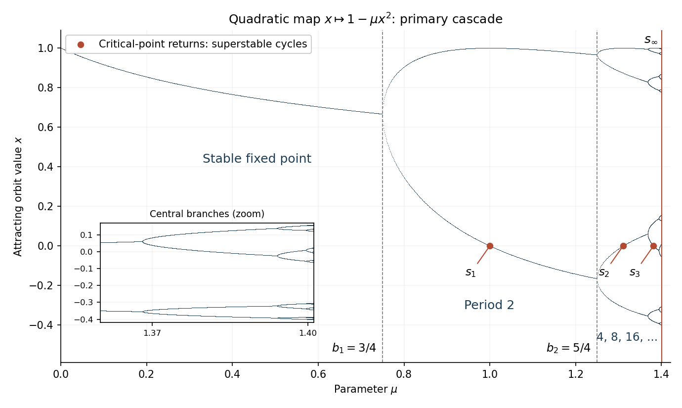
For the quadratic unimodal map, an attracting fixed point lies on the positive branchIts multiplier has modulus less than one for $0\le \mu <3/4$ and reaches $-1$ at the first period-doubling bifurcation $b_1=3/4$. The resulting two-cycle has pointsIts periodic-orbit multiplier is $4{\mu }^2{x}_{+}{x}_{-}=4(1-\mu )$, so it is attracting for $3/4<\mu <5/4$ and doubles at $b_2=5/4$. Successive attracting periods are $4,8,16,\dots$, with their parameter intervals shrinking toward $s_{\infty }\simeq 1.401155189$.

A superstable periodic orbit contains the critical point zero, so its derivative product vanishes. Along the first period-doubling cascade, $s_n$ is the first-cascade parameter with a critical orbit of exact period $2^n$, satisfying $f_{s_n}^{2^n}(0)=0$. For example, $s_1=1$, $s_2\simeq 1.310702641$, and $s_3\simeq 1.381547484$. These are interior points of stability intervals, distinct from the bifurcation parameters $b_n$.

The following bifurcation diagram shows attracting orbit values, including the first bifurcations and superstable points. At the accumulation parameter the limiting critical orbit is not a finite attracting cycle; its closure is the period-doubling limit set.

The Feigenbaum constants use the positive spatial-scaling convention. Their parameter definition isThe same limit is obtained from successive bifurcation parameters. To define spatial scaling without ambiguity about signs, letThis is the signed central return separation in the superstable $2^n$ orbit; its sign alternates between successive levels of the primary cascade. ThenEquivalently, the ratio of the corresponding unsigned separations tends to $\alpha$. Some conventions call the signed ratio itself $\alpha$; here the spatial scale of the Feigenbaum renormalization fixed point is $a=-1/\alpha <0$, matching the orientation reversal in the doubling operator.

The normalization fixes the critical point at zero and its image at one. It removes arbitrary height and spatial scales, so successive renormalized return maps can be compared in one function space rather than drifting through rescaled copies of the same dynamics. The second iterate near the critical point has a minimum; a negative rescaling reverses it back to a maximum.

Because $f(0)=1$, the period-doubling renormalization operator satisfiesPreservation of normalization therefore forcesThe scale is a functional of $f$, not an independently adjustable constant. In the renormalizable regime it lies in $(-1,0)$. If $h(x)=ax$, then $\mathcal{T}(f)=h^{-1}\circ f^2\circ h$ on the central restrictive interval. Thus topological conjugacy relates one iteration of the renormalized map to two iterations of the original map, and the new critical value is again one. For $f_{\mu }$, $a=1-\mu$, so this regime starts beyond the superstable two-cycle at $\mu =1$.

Normalization alone does not make every normalized unimodal map renormalizable: the central interval and its image must form the appropriate period-two restrictive pair, so that the rescaled second iterate is again an even unimodal map into $[-1,1]$. The operator is considered on the neighbourhood where these additional conditions hold.

Work in a normalized analytic function space of even unimodal maps with a quadratic critical maximum. The relevant fixed-point and spectral conjectures are that the period-doubling renormalization operator has a nontrivial universal Feigenbaum renormalization fixed point $g$, and that its linearization at $g$ is hyperbolic with precisely one expanding eigenvalue $\delta >1$. Its remaining spectral directions contract. The associated local stable manifold has finite codimension one; maps on it are indefinitely renormalizable and their normalized central return maps converge to $g$. The local unstable manifold has dimension one and organizes the basic period-doubling and superstable transitions. These assertions concern the normalized quadratic universality class, rather than arbitrary functions or every parameter family.

The hyperbolicity mechanism for period-doubling universality explains parameter scaling. Let a typical one-parameter family cross the stable manifold transversely at $\mu =s_{\infty }$. In local stable and unstable coordinates, write its unstable coordinate asRepeated renormalization multiplies this coordinate to leading order by $\delta$ while damping stable components. A superstable orbit of period $2^n$ becomes a superstable two-cycle after $n-1$ renormalizations. Hence its parameter is characterized by arrival at the same basic superstable surface, at a fixed nonzero unstable coordinate after the initial transient. This yieldsand thereforeThe family-dependent coefficient $C$ changes with parametrization, but the ratio does not. The same argument applies to the primary bifurcation surfaces and their successive preimages. Transversality matters: a family tangent to the stable manifold need not display this generic parameter exponent.

Spatial universality follows from the fixed point's scale $a_g=g(1)<0$. As renormalized maps approach $g$, their successive central restrictive intervals shrink by factors approaching $|a_g|$, with orientation alternating. Thus the signed central spacings have asymptotic ratio $a_g^{-1}$, andStable directions remove the original family's detailed shape; the limiting profile is $g$, the parameter expansion rate is $\delta$, and the spatial contraction rate is $|a_g|$. Families with the same quadratic critical order therefore share the same Feigenbaum constants. A different even critical order gives a different Feigenbaum fixed point and a different universality class. This explanation is a consequence of the fixed-point, hyperbolicity and transverse-transition properties; it is not a proof that an arbitrary one-parameter family satisfies those properties.

Write the local Taylor series at the critical point aswhere $d$ is even, and put $a=g(1)$. The fixed-point equation first gives $g(g(0))=g(1)=a$, consistently with normalization. Expanding the inner function at zero and the outer one at one,The quadratic remainder in the outer expansion is of order $x^{2d}$, at least $x^{d+2}$ because $d\ge 2$. Comparing the nonzero $x^d$ coefficients proves the exact identityTo obtain the requested first-order relation, use the leading polynomial approximation to a renormalization fixed point: retain only $g(x)\approx 1+c{x}^d$. Then $a\approx 1+c$, while $g^{\prime }(1)\approx dc$, giving the truncated equationThe equality belongs to this truncation; higher analytic coefficients generally change $g^{\prime }(1)$ and $a$, so it is not an additional exact equation for the full fixed point.

For $d=2$, solve $2a(a-1)=1$. The root compatible with $-1<a<0$ is $a=(1-\sqrt{3})/2$; the other root is inadmissible. ThusThis is a coarse leading approximation, not the more accurate universal value $2.5029\dots$ obtained after retaining higher coefficients.

At a current approximation $p$, Taylor's theorem replaces $\Phi (p+h)=0$ by the affine equation $\Phi (p)+D\Phi (p)h=0$. Solving this equation gives the Newton iteration in a Banach spaceThe inverse is a bounded linear inverse by the bounded inverse theorem. The displayed operator is defined where the derivative is invertible, in particular on the specified open domain; the hypotheses do not supply a globally defined Newton operator on all of $\mathcal{X}$. If $\Phi (\bar{p})=0$ with $\bar{p}$ in that domain, then $N(\bar{p})=\bar{p}$.

For quadratic convergence, choose a sufficiently small neighbourhood of $\bar{p}$. Continuity of the inverse derivative and of $D^2\Phi$ gives constants $M,L$ there such thatPut $e=p-\bar{p}$ and $B(p)=[D\Phi (p){]}^{-1}$. The quadratic Newton error bound in a Banach space follows from the integral remainder:soTake a closed radius-$r$ ball lying in the neighbourhood with $Cr<1$. This inequality maps the ball into itself and makes errors tend to zero. More explicitly, for $e_n=\Vert p_n-\bar{p}\Vert$, induction gives $C{e}_{n+j}\le (C{e}_n{)}^{2^j}$. Hence every sufficiently close initial point converges to $\bar{p}$ at least quadratically; special maps can converge still faster.

For a fixed-point equation, apply the same method to $F(p)=\Phi (p)-p$. Wherever $D\Phi (p)-I$ is invertible, the exact adapted map isEvery fixed point of $\Phi$ is fixed by $A$, and conversely on this domain. This additional invertibility condition is distinct from invertibility of $D\Phi$; for example, $D\Phi =I$ is invertible but $D\Phi -I=0$ is not.

For certification, a frozen Newton correction for a fixed-point equation is often more useful. Choose a bounded, injective approximate inverse $J$ of $D\Phi (p_0)-I$ and setAgain $A_J(p)=p$ if and only if $\Phi (p)=p$. A well-chosen $J$ makes the corrected operator contract even if the original operator has an expanding direction. The subsequent contraction mapping argument requires the stated derivative and residual bounds; it does not assume that arbitrary inverse approximations provide them.

Let $B=\{p:\Vert p-p_0\Vert \le r\}$ and write $\epsilon =\Vert A(p_0)-p_0\Vert$. Integrating the Fréchet derivative along the line segment between two points in the convex set givesand the operator norm bound impliesIn particular, for $p\in B$,Thus the a posteriori contraction ball is mapped into itself. The ball is a closed subset of a Banach space, hence is a complete metric space. Applying the contraction mapping theorem to $A:B\to B$ gives existence and uniqueness:The estimate also gives $\Vert p_{\ast }-p_0\Vert \le \epsilon /(1-\kappa )$, by applying the same triangle inequality to $A(p_{\ast })=p_{\ast }$. Equality in the residual bound is allowed; strict contraction mapping comes from $\kappa <1$, and a fixed point on the closed ball's boundary is included.

The Lanford contraction proof of the Feigenbaum fixed point replaces an unstable renormalization operator by a contracting Newton correction. Use a coefficient Banach space for normalized even maps, represented by $p(x)=1-x^{2}h(x^2)$ with an absolutely summable coefficient norm on $h$. Its complex domain and a small ball are chosen so that every map is admissible and the renormalization composition is analytic there.

A high-accuracy polynomial $p_0$ gives an approximate fixed point. Use a bounded invertible approximate inverse $J$ for $D\mathcal{T}(p_0)-I$, and defineRigorous estimates certifyThe finite coefficient computations use interval arithmetic with controlled rounding; analytic estimates bound the infinite tail. Thus the certification applies to the full function space, rather than merely a truncated polynomial system.

Part (b) gives a unique fixed point of $A$ in the certified ball. Invertibility of $J$ makes it a unique fixed point $g$ of $\mathcal{T}$ there. The ball also preserves the quadratic critical maximum and nontrivial shape, excluding the constant formal normalized solution. Consequently an actual locally unique analytic Feigenbaum fixed point exists, with the error bound $\Vert g-p_0\Vert \le \epsilon /(1-\kappa )$. The numerical approximation locates it; rigorous residual, derivative and tail bounds establish its existence and uniqueness. This conclusion is local, not a claim of global uniqueness among all analytic solutions.