Let be kinematic pressure, with the resting hydrostatic part subtracted, and let be the buoyancy perturbation about background buoyancy . The nonrotating inviscid Boussinesq equations, with no buoyancy diffusion, areHere the third equation is mass conservation for incompressible flow, and the last expresses buoyancy conservation following a parcel. Linearization about rest removes the products of disturbances. For a plane internal gravity wave proportional to , the resulting Linearized Boussinesq equations becomeWith and , the first and third equations give . Substitution in vertical momentum and buoyancy gives the dispersion relationSince the velocity is the time derivative of the displacement field, . Thus the complete buoyancy polarization of a plane internal gravity wave isBoth velocity and displacement are perpendicular to the wavevector; pressure and velocity are in quadrature with buoyancy and displacement.
For upward/rightward phase velocity, choose and . Differentiating this dispersion relation gives the group velocity, while the vector phase velocity points along the wavevector:Their dot product is zero and . Draw from the tip of : the right-triangle geometry of internal-wave velocities has horizontal hypotenuse . This hypotenuse is distinct from the horizontal phase velocity .
At an instant with real complex amplitude , write . The spatial fields areThe constant-phase lines of an internal gravity wave slope down to the right, with . Buoyancy maxima lie a quarter wavelength from pressure maxima; the oscillating displacement and velocity run along the phase lines. The group velocity points down and right along them, despite upward/rightward motion of the wave phase.
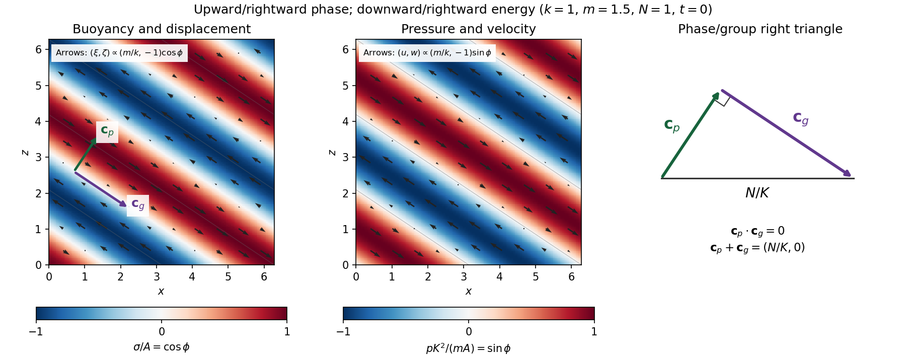
Internal-wave buoyancy, displacement, pressure and velocity fields, with downward energy propagation and the phase/group-velocity right triangle
. Details. 
Let , using horizontal averaging over a wavelength. This is the displacement pseudomomentum of an internal gravity wave, whose sign convention is opposite to . For complex coefficients, . The above wave polarization consequently givesSince , these obey . With weak kinematic viscosity, each leading monochromatic velocity component satisfies , . The dissipative term is therefore , so the supplied averaged balance reduces toFor constant and a steady wave envelope, . As is proportional to squared wave amplitude, viscous attenuation of an internal gravity wave givesHere , so amplitude decreases below a source at : the source is above the receiving level. The same conclusion follows directly because downward group velocity carries energy from the source downward. Upward phase velocity does not locate the source.
For a slowly varying mean shear flow , the local intrinsic frequency is . A local WKB approximation uses , with varying vertical wavenumber and group velocity. The appropriate transported quantity is wave action, or horizontal wave pseudomomentum ; its vertical flux has viscous loss, and the changing polarization factors must be retained. In particular, is no longer constant.
Near a critical level of an internal gravity wave, , so and . The damping per vertical distance, of order , grows rapidly. The waves are strongly attenuated over a narrow altitude range and transfer momentum to the mean flow there or before reaching the critical level. The inviscid WKB approximation eventually fails; viscosity and possibly internal-wave breaking regulate the small scales.
Let be layer thickness and gravitational acceleration. The unforced shallow water equations on the equatorial beta plane areLinearize about , . Put and , and scale , , and . Dropping capitals, the linearized shallow water equations becomeThe choice makes both the wave speed and the coefficient of the dimensionless Coriolis parameter equal to one.
Take Fourier modes that decay as . Their equations areFor and nonzero , the first two require . The root gives , and meridional balance becomes . Hence the equatorial Kelvin wave isIt travels eastward at speed in dimensional units. The other sign gives and , so is not trapped.
For , and , inversion of the first two equations gives the equatorial wave velocity polarizationSubstitute in the remaining momentum equation. Multiplication by leavessoWriting yields , the Hermite differential equation. The trapped solutions have the Hermite oscillator quantization and .
For completeness, quantization follows without assuming that every acceptable solution is a polynomial. On decaying smooth functions, define , and . Integration by parts gives and . If , it is an eigenfunction of with eigenvalue . Repeated lowering must terminate: otherwise it eventually produces an eigenvalue below one. At termination , so the terminal eigenfunction is and has eigenvalue one. Repeated raising gives and ; uniqueness of a decaying solution at one end of this second-order equation fixes each mode up to scale.
Thus, away from the exceptional quotients, all fields are determined byInsert this and its derivative in the polarization formulae to obtain and . For , the cubic supplies the low-frequency equatorial Rossby wave and two equatorial inertia--gravity wave branches. Their meridional structures are Gaussian-weighted Hermite polynomials.
For , multiplication by factorizes the equatorial shallow-water dispersion relation asThe physically admissible quadratic gives the mixed Rossby-gravity wave, equivalently the Yanai wave:These fields satisfy all three original equations directly and decay at both infinities, including where the quotient formulae are singular.
To test the other factor, set . The original equations give and . Put ; meridional momentum then givesDecay of at both infinities requires the integral of the right side to vanish. Hence unless . Ordinarily the extra factor supplies no trapped mode. At the exceptional root of the mixed Rossby-gravity mode, , it coincides with the quadratic root and gives the same physical fields, not an additional branch. This distinction avoids discarding a regular physical mode at the crossing.
These arguments concern nonzero wave angular frequency. At , the oscillatory nonzero- modes have , while zero-frequency geostrophic states must be considered in the original equations rather than in expressions divided by .
The basic quasi-geostrophic streamfunction gives , and constant quasi-geostrophic potential vorticity . DefineBecause the background has no potential-vorticity gradient, the linear potential-vorticity equation is simplyIts characteristics have constant , so the general solution is . In particular, is the requested arbitrary separated family; one product is not the most general initial field.
Linearizing the vertical velocity requires retaining advection of by . ThereforeThe impermeable boundary at imposesThis is conservation of boundary buoyancy, not merely a condition that vanish.
For zero interior potential vorticity, write . With , stratified quasi-geostrophic inversion givesThe decaying solution isNo time dependence has been assumed to obtain this vertical structure. Applying the boundary condition gives , henceThus the Eady edge wave travels eastward with horizontal phase velocity for .
The propagation mechanism can be made explicit using boundary parcels. Thermal wind gives the background buoyancy gradient . A small meridional parcel displacement produces boundary buoyancy perturbation . Meanwhile the decaying potential-vorticity inversion gives at the boundary. Consequently there, and the parcel equation becomesA displaced buoyancy contour therefore induces a velocity field that advances that displacement eastward. No interior potential-vorticity gradient is needed because the boundary buoyancy supplies the invertibility data.
Vortex stretching is what sets the induced flow's vertical reach. In the interior, the zero-potential vorticity condition requiresBoundary isopycnal displacement decreases with height as , so fluid columns are stretched or compressed over depth . Conservation of potential vorticity makes this stretching balance the relative vorticity. The resulting inversion factor gives the propagation speed: stronger density stratification reduces penetration and speed, while larger increases them. Zero interior potential vorticity therefore does not imply zero interior flow.
For imposed boundary vertical velocity, retain the same decaying structure and writeThe boundary relation becomes the forced Eady edge wave equationThe integrating factor gives, for ,The arbitrary homogeneous coefficient sets the initial disturbance. With , this is .
At resonance, , integration instead yieldsAn initially undisturbed fluid has . The imposed pumping reinforces the same boundary normal mode every cycle, with no dissipative loss, so the linear amplitude grows secularly. The divergence describes resonance of the undamped linear model; sufficiently large wave amplitude invalidates the assumed small-disturbance approximation.
Potential-vorticity inversion is the diagnostic recovery of the flow from its advected vortical scalar, using the balance relation and specified boundary conditions. Its usefulness is a separation of tasks: transport the scalar by the current velocity, invert to find the new velocity, and repeat. The inverse is spatially nonlocal even though the transport law is local. The four models differ chiefly in the operator being inverted and the information needed at boundaries.
In two-dimensional vortex dynamics, planar incompressibility permits , and vertical vorticity is . The curl of inviscid momentum givesThere is no vortex stretching in strictly planar motion, so vorticity is materially conserved. The two-dimensional potential-vorticity inversion is the Poisson equation . On the plane, with suitable integrability and far-field behavior, its Green's function is , givingDifferentiation gives the planar Biot-Savart kernel. Here is a harmonic function fixed by boundary, circulation and far-field data. A rigid impermeable wall is a streamline, so is constant on it; constants or circulations around distinct holes require specification. The vorticity alone cannot distinguish two flows differing by a permitted harmonic contribution, such as a uniform current on an unbounded plane. A constant added to has no physical effect.
In nonrotating layerwise-two-dimensional vortex dynamics, strong stable density stratification constrains motion to almost horizontal layers. In the ideal independent-layer limit, vertical velocity vanishes at leading order, andhold separately at each fixed . Height is a parameter: the horizontal inverse Laplacian contains no vertical derivative. With background buoyancy , the leading Ertel potential vorticity is , so the materially advected normalized scalar is . The same horizontal Poisson equation is inverted layer by layer, using each layer's boundary data. This is an asymptotic constrained model, not arbitrary three-dimensional Euler motion with vertical velocity set to zero: its validity requires small Froude number and controlled vertical scales. At finite buoyancy frequency, the weak vertical motion and tilted isopycnals restore coupling. The inversion may be independent by layer while the reconstructed fields vary with height. The horizontal Euler equations for an inviscid fluid determine the pressure gradient, while hydrostatic balance relates its vertical derivative to buoyancy.
In shallow-water quasi-geostrophic inversion, begin with the exact shallow-water potential vorticity . Linearizing its anomaly about depth gives, after multiplying by , . For small Rossby number, geostrophic balance gives , while . Keeping the beta plane background gradient givesThus is inverted with the modified Helmholtz equation , under the specified boundary and far-field conditions. The velocity follows from and surface elevation from . A horizontal Fourier mode of the anomaly satisfiesThe Rossby deformation radius therefore limits the reach of the balanced response. Layer stretching, represented by , is absent from ordinary planar vorticity inversion. Unlike the pure Poisson equation, the finite-deformation operator also responds to the constant part of , which specifies mean elevation rather than an arbitrary streamfunction offset. Specified bottom topography adds a known source to ; it is subtracted along with the background before inversion.
In stratified quasi-geostrophic inversion, continuously varying vertical displacement replaces the shallow layer's single stretching term. For positive and constant nonzero , the three-dimensional quasi-geostrophic potential vorticity isGeostrophic balance and hydrostatic balance give velocity and buoyancy perturbation . Invert the anisotropic elliptic boundary value problem using interior , prescribed top and bottom buoyancy as Neumann boundary conditions, and the lateral, far-field and global-flow data. Boundary buoyancy evolves by its own material conservation when the boundary is impermeable. It cannot be discarded: the Eady edge wave in the preceding solution has zero interior potential vorticity anomaly but nonzero boundary buoyancy and a nonzero induced flow.
For constant , the stretched coordinates for quasi-geostrophic inversion turn the inversion operator into the three-dimensional Laplacian. Its infinite-space Green's function is in coordinates. Hence a horizontal disturbance of scale communicates vertically over scale , explicitly coupling layers. In a bounded domain with homogeneous difference data, multiplying the difference of two inversions by its streamfunction and applying integration by parts givesThis proves uniqueness up to a constant when the relevant boundary terms vanish; a mean or pressure reference fixes the remaining constant. Compatible boundary fluxes are needed for a purely Neumann boundary-value problem.
Across all four models, inversion provides the induced flow, while scalar transport supplies time evolution. The independent horizontal inverse in the first two models becomes a finite-deformation inverse in shallow water and a vertically coupled elliptic inverse in continuous stratification. The principle applies within the stated balance or constrained model. In the unrestricted Boussinesq equations or shallow water equations, gravity waves and divergent motion can share the same potential vorticity, so the vortical scalar alone does not reconstruct every possible flow.
Articles by others on the same topic
There are currently no matching articles.