Put and impose homogeneous Dirichlet boundary conditions, as required by the stated continuum eigenvalues. Let be the unscaled one-dimensional Dirichlet discrete Laplacian. For , the vectors satisfyThe identity follows by adding the two neighboring sines; the values at vanish. These mutually orthogonal vectors form the discrete sine transform basis. Consequently their tensor products give all two-dimensional modes, not merely a few candidate eigenvectors.
In a compatible grid ordering the axial operator is . The nine-point operator isIndeed, the added Kronecker product supplies the diagonal neighbors with weight , subtracts from each axial neighbor and adds to the central coefficient. Thus it has exactly the coefficients of the second discretization. On the eigenvalues areandEquivalently, .
For fixed mode numbers , expansion of the sines giveswhereas the mixed Kronecker product correction givesThus both eigenvalue approximations are second order for fixed modes. The leading nine-point error includes an additional positive term .
There is also an exact comparison, not just an asymptotic one. Since for , and both sine factors in the correction are positive,Both estimates lie on the less-negative side of the continuum Laplacian eigenvalue, so the five-point formula is the better eigenvalue estimate for every corresponding interior mode. The five-point versus nine-point Laplacian eigenvalue accuracy comparison does not contradict the useful isotropy or special Poisson accuracy properties of a nine-point stencil. Those properties concern a different error criterion. The fixed-mode expansion is not uniform for modes with or comparable to ; wavelengths close to the mesh scale need not have small relative spectral error.
Work in the standard class of real constant-coefficient linear multistep methods using only first-derivative evaluations. Writewith . The Dahlquist equivalence theorem states that such a method converges on each fixed finite time interval, for sufficiently regular Lipschitz initial value problems and every set of consistent starting values, if and only if it is consistent and zero-stable. Consistency means and . Zero-stability means all roots of lie in and every root on is simple. In particular the consistency root at is simple.
Taylor expansion of the exact-solution residual gives the exponential-symbol order criterion for a multistep methodThis criterion packages the identities through . We now derive the upper bound on from the root condition, rather than assuming the first Dahlquist barrier.
Use the Cayley transform and defineThe simple root at gives , while and . Each finite transformed root is , with nonpositive real part when . A possible root at simply lowers the degree of . Factor over the reals: a real root contributes with , and a conjugate pair contributes with . Therefore, after reversing the overall sign if needed,Since , the order criterion is equivalent toThe key coefficient sign lemma for the first Dahlquist barrier isHere is a proof of that sign assertion. Direct integration givesDifferentiate twice and pair the terms at and to obtainThe power series of has positive odd coefficients. The even powers in the hyperbolic cosine therefore have nonnegative coefficients, and has strictly positive even coefficients. Every even coefficient of is consequently negative. Also is even and , proving the assertion.
If is odd and , the coefficient of in must vanish because . But it iswhere out-of-range indices are zero and the sum includes the strictly positive . This is impossible, so . If is even and , exactly the same argument with the coefficient of gives a contradiction. Thus in that case. This proves the Cayley coefficient proof of the first Dahlquist barrier:To prove that the bound is attainable for every , let be the Lagrange polynomials for the nodes , and take . The Newton-Cotes multistep methods attaining the first Dahlquist barrier areThe underlying Newton-Cotes closed quadrature is exact on all polynomials of degree at most . For even , the node polynomial is odd about , so . Dividing any degree- polynomial by shows that quadrature exactness extends one degree further. Integrating the exact derivative therefore gives method order at least for odd and at least for even .
Finally has only simple unit-circle roots, so these methods satisfy the root condition. The weights sum to , proving consistency. The Dahlquist equivalence theorem gives convergence with consistent starts; the proved upper bound makes the attained formal orders exact; starting values accurate to those orders also give the corresponding global accuracy. Hence the highest convergent order is . This result concerns the stated linear first-derivative class, not unrestricted multiderivative or nonlinear formulas.
Let be the vector of ones. For a general nonautonomous Runge-Kutta method the stages satisfy and the update is . Expansion at givesand thereforeThe exact solution is . Matching the independent terms gives the necessary and sufficient second-order conditions with independent Runge-Kutta abscissaeUnder the usual internally consistent Butcher tableau convention , this reduces to , , . If the abscissae are allowed to be independent of the row sums, is a sufficient simplifying convention rather than a logically necessary order-two condition.
The original PDF has a sign defect in the lower-left stage coefficient. Put . With the printed negative sign, the row sums and the relevant Butcher order conditions areThus the claimed universal second order is false. For example gives, on , two stages equal to and the update . This is the first-order Forward Euler method. For the literal tableau, order at least two holds exactly when or , subject to distinct allowed nodes.
For completeness the literal tableau's A-stability can also be classified algebraically. DefineThe stability function obtained from isIf , the denominator has no zero in the closed left half-plane: its reciprocal roots are the stage-matrix eigenvalues, whose positive sum and nonnegative product give positive real parts for nonzero eigenvalues. On the imaginary axis,Consequently for the literal tableau with uniquely solvable stages throughout the left half-plane, the complete parameter criterion isThese explicit inequalities in are necessary by the small and large imaginary parameters, and sufficient by the maximum modulus principle, including the bound at infinity. For the last inequality forces , leaving the stable linear-fractional case. For there is a negative real stage pole. If one defines stability solely through an analytically continued scalar stability function, the only additional possibilities areIndeed these are precisely the cases where the left pole cancels and is an A-stable theta method. The original stage equations are nevertheless singular at , so they do not give uniquely determined stages there. This distinction prevents a canceled rational factor from concealing an ill-defined stage solve.
The natural intended repair is to replace just the lower-left coefficient by . This makes the method the collocation Runge-Kutta method on the two nodes. To derive the repaired entries, takeIntegration gives the other three printed entries and the weights unchanged, with the positive lower-left entry. Since and , it follows that , and . Hence the corrected family is always of order at least two.
For the corrected family let , and . Its stability function has the same displayed rational form, now with . The denominator again has no left-half-plane zero, and on the imaginary axis the squared-modulus difference is . Because , the necessary and sufficient inequality is , orFor sufficiency, on the imaginary axis and at infinity; apply the maximum modulus principle on growing left half-discs to get the same bound inside. If , the condition leaves the endpoint trapezoidal rule and its linear denominator. If , every nonzero imaginary argument gives . This is the two-node collocation A-stability criterion, explicitly distinguished from the literal defective tableau.
Expand the three matrix exponentials and retain terms through degree two. Their product iswhich agrees with to that order. Keeping the cubic terms gives the more informative defectwhere is the commutator. For example, the coefficients of in the product are , instead of the exact . The cubic defect is generically nonzero. Therefore Strang splitting has order . The symmetry is consistent with this cancellation of the quadratic defect; for commuting the composition is exact rather than merely second order.
Choose the centered Dirichlet discrete Laplacian in each direction. With put , and . Thus and are the physical derivative approximations; the factor has been absorbed into the Courant number in the written update. Equivalently use the scaled derivative matrices and the time parameter .
For a one-dimensional vector with endpoint values ,Thus and are real symmetric negative-definite matrices. An orthonormal eigenvector basis shows that all eigenvalues of each exponential lie in for , soIterating gives for every nonnegative step parameter, a mesh-independent unconditional stability bound. Multiplying the squared norm by the grid-area weight leaves the same estimate. In this natural tensor-grid choice , so : the split update is even the exact semidiscrete diffusion flow. Contractivity of a product of these negative symmetric exponentials would prove stability even without commutation.
Write , . Every smooth exact solution of the advection equation here is . At , substitution into the scheme gives the unscaled residualThe constant, linear and quadratic Taylor coefficients vanish. Its cubic coefficient isFor a general smooth function the first-order residual is , so the proper normalized local truncation error on an exact solution isHence the scheme has formal order two for fixed general positive . At and , the displayed residual vanishes identically for every , not just to one higher Taylor order: the recurrence transports exactly sampled characteristics when both starting levels are compatible with the exact solution. This formal exactness does not imply stability. At there is no positive time step. The two-level recurrence also requires a starting procedure for ; one initial solution profile alone is not two independent starting levels.
Insert a Fourier mode . With and , the amplification polynomial isIts two roots have product , of modulus one. Thus if both roots are bounded by one, both must have modulus exactly one. Set . The equation becomesWhen , both roots have modulus one and their separation obeys for every frequency. The companion matrix has bounded entries and can be diagonalized with the two eigenvectors . The uniform separation bounds the inverse eigenvector matrix. Hence every matrix power is bounded uniformly in and , and the Parseval identity proves L2 norm stability for the two starting levels on the whole grid.
If , frequencies near give one root outside the unit circle, so the scheme is unstable. If , the Nyquist polynomial is , a repeated unit root. The corresponding companion matrix has a nontrivial Jordan block and solutions containing . Thus the endpoints are unstable as well. On the whole line the individual Nyquist plane wave is not square-summable, but Fourier packets localized arbitrarily close to that frequency realize the unbounded power norm by continuity. Therefore the uniform stability of a shifted two-level advection scheme criterion isIn particular is stably exact with compatible starts, whereas is formally exact but unstable under arbitrary perturbations. Checking only the moduli of the roots and retaining both endpoints would miss this essential distinction.
Sparse Gaussian elimination seeks a direct solution while preserving the advantage of a small number of nonzeros. The main issue is that eliminating unknowns creates new interactions between the remaining unknowns. For a symmetric positive-definite system, simultaneous row and column permutation merely changes the elimination order, and Cholesky decomposition or LDL decomposition can proceed without pivoting. Partition one elimination step asThe remaining system has the Schur complement . It is positive-definite because, for any nonzero , minimizing the positive quadratic form of over the first coordinate gives . This both justifies the next positive pivot and identifies exactly where fill can appear.
The matrix graph of a symmetric sparsity pattern has one vertex per unknown and an edge when is structurally nonzero. At pivot , the updatecan change an entry only when both and are current neighbors of . Thus the elimination graph operation removes and makes its remaining neighbors a clique. Edges absent before this update are fill-in. The graph describes structural or generic nonzeros: special cancellations in the numerical values can reduce the actual fill, but cannot justify omitting possible entries in advance.
A useful global description is the fill-path criterion for symmetric elimination. After a set has been eliminated, remaining vertices are adjacent generically exactly when their original graph contains a path from to with all internal vertices in . The assertion starts with the original edges when is empty. Eliminating the next vertex concatenates two earlier such paths through it; conversely, split any allowed path at the newly eliminated vertex to recover the two earlier connections. This induction explains why sparse long-range couplings may eventually become dense.
The order is decisive. For a star with four leaves, eliminating a leaf only changes the diagonal of its sole neighbor and creates no fill. Repeated leaf elimination preserves this property. Eliminating the central vertex first instead connects all four leaves, creating six edges and a dense four-variable trailing system. This occurs, for example, in a positive-definite star matrix with central diagonal , leaf diagonals and edge entries ; no cancellation removes the new leaf couplings.
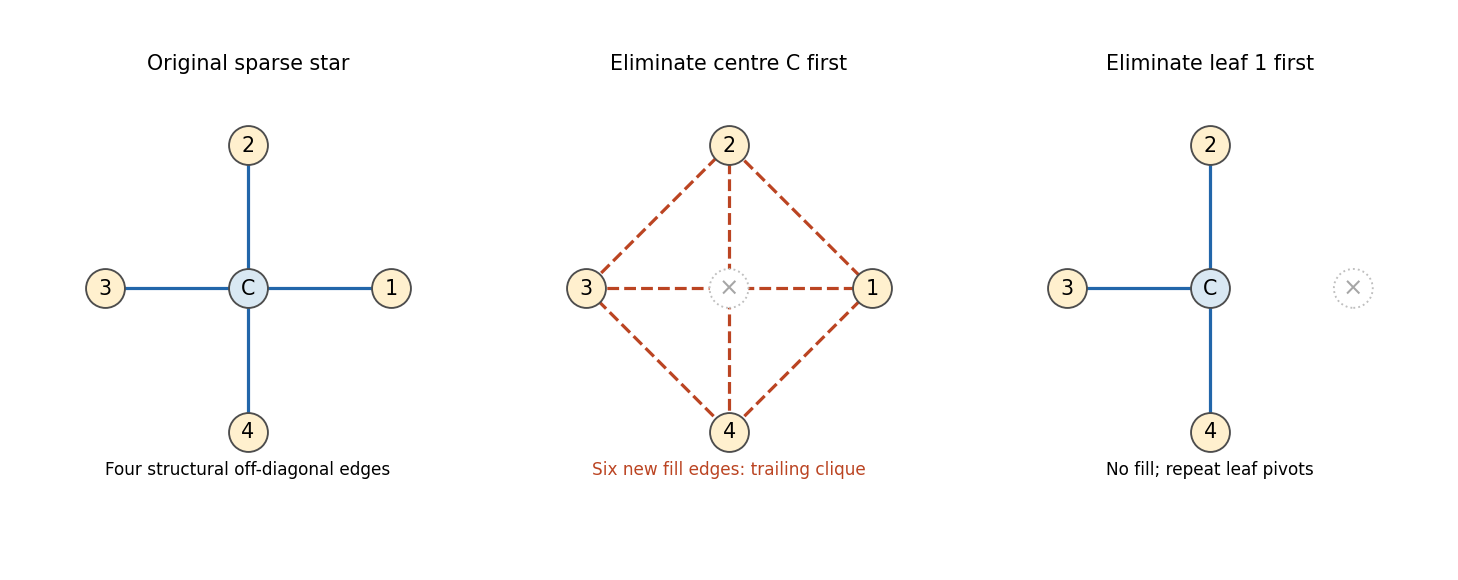
The same sparse star graph creates no fill with leaf elimination and six fill edges with central elimination
. Details. 
For an arbitrary graph, an ordering creates no fill precisely when each pivot's later neighbors are already a clique, namely a perfect elimination ordering. Such an ordering exists exactly for a chordal graph. A chordless cycle of length at least four illustrates the obstruction: its first removed vertex connects its two previously nonadjacent neighbors. Eliminating in a chosen order adds chords until the completed graph is chordal. Thus sparsity of the original matrix alone does not guarantee sparse factors; the graph and its ordering matter together.
If pivot has later neighbors, its column contains factor entries and its symmetric outer-product update costs arithmetic. The total storage is governed by and the work by . A band ordering with matrix bandwidth gives the familiar storage and work, but a narrow profile or graph separator can do better than a single global band. The minimum degree algorithm greedily chooses a current low-degree pivot; it often keeps immediate updates small, but it must account for previously created fill and need not minimize total fill.
Nested dissection instead finds a small vertex separator, recursively eliminates disconnected subdomains, and leaves separator variables until last. For a regular two-dimensional grid with unknowns, a separator has vertices. Its dense final work is , and recursive balanced separation givesAt each level the summed separator-square storage is , giving factor storage over the logarithmic number of levels. These estimates assume the usual geometric separator structure; they are not guarantees for every sparse graph. Independent subdomains also expose parallel work.
In a practical solver a symbolic factorization phase uses the pattern and ordering to allocate factor storage and schedule updates. For the lower-triangular factor, the elimination tree takes the parent of column to be its first later row index containing a structural nonzero. Descendant updates flow towards those later pivots, making the tree useful for dependency scheduling and the organization of the factorization. Compressed sparse storage records only entries and indices; the numerical phase then computes the values, followed by forward and backward substitution. The factors can be reused for many right-hand sides.
Finally, structural efficiency must be balanced with numerical stability. For a nonsymmetric system the pattern can be represented by a directed or bipartite graph, and elimination creates edges from incoming to outgoing neighbors. Separate row and column permutations are possible. A fill-reducing column ordering does not ensure a safe pivot: scaling and partial pivoting may be needed to prevent division by a tiny number and large growth. Such row interchanges can change the predicted fill. Positive-definite symmetric problems avoid this conflict; general sparse solvers must manage it explicitly. Graph-based ordering controls factor sparsity, while pivoting controls numerical safety; an effective sparse factorization needs both.
Stability of a numerical method controls how perturbations in initial data, roundoff and local residuals propagate. For a linear evolution scheme , a suitable finite-time requirement iswith independent of the refining mesh. The norm should approximate the norm of the continuous problem, such as an area-weighted L2 norm. The bound need not imply decay: is appropriate when the equation itself permits finite-time growth. For a multilevel scheme the state includes all required time levels.
The error recurrence shows why stability matters. If , thenThus a consistent residual tending to zero and a convergent start produce convergence when the stability constant is uniform. Tiny defects need not remain tiny without that bound. The Lax equivalence theorem makes this precise: for a well-posed linear initial value problem and a consistent linear approximation, stability is equivalent to convergence in the compatible solution norms. It is not a theorem for arbitrary nonlinear schemes, and a high formal order does not substitute for stability.
For constant coefficients on a periodic or infinite grid, von Neumann stability analysis diagonalizes spatial translations using Fourier modes. If , the Parseval identity converts a uniform multiplier-power bound into an L2 norm bound. The contraction condition is sufficient; a more general also yields a finite-time bound. For the centered-space explicit heat method,so exactly for . Larger fixed Courant numbers amplify high frequencies. The Backward Euler method gives instead and is contractive for every .
For , forward time and centered space give , with . Hence for nonzero frequencies, causing instability at a fixed nonzero Courant number. The directionally correct upwind finite difference scheme uses the neighbor at and hasIt is contractive exactly for . This also has a direct maximum-norm proof: the update is a convex combination of two old values. The continuum domain of dependence must fit inside the numerical one for a local explicit hyperbolic method to converge, giving the Courant–Friedrichs–Lewy condition. That necessary geometric restriction is not by itself a sufficient stability proof.
For systems and multilevel methods, each Fourier multiplier becomes a matrix. All amplification roots must obey the appropriate root bound, but their moduli alone are insufficient. A repeated unit root in a companion matrix gives a Jordan block; for instance has . Even distinct roots require control of the diagonalizing matrices uniformly in frequency and mesh. The uniform power bound from separated amplification roots supplies such control for a bounded two-root family with a positive gap. Question5 illustrates both sides: strict gives a uniform gap, whereas the endpoints have a double unit root and are unstable despite unit moduli.
Energy estimates are especially useful when coefficients vary or boundaries prevent Fourier diagonalization. As a simple example, for implicit heat evolution with homogeneous Dirichlet boundary conditions, take the grid inner product of with . Discrete integration by parts givesThe boundary term vanishes because the boundary values are zero, proving contraction. For variable positive diffusion coefficients the corresponding flux-weighted squared differences remain nonnegative, so the argument extends without a constant-coefficient Fourier symbol. With forcing or lower-order terms, a discrete energy inequality and Gronwall inequality yield a mesh-independent finite-time bound.
A related technique is eigenvalue stability analysis of a finite difference method. If the spatial matrix is symmetric with nonpositive eigenvalues and the time update is , an orthonormal eigenbasis givesThis proves stability when all scaled spatial eigenvalues lie in the time method's stability domain. For a nonnormal spatial or amplification matrix, the eigenvalues alone do not control powers: ill-conditioned eigenvectors or Jordan terms can cause transient growth. Direct operator-norm estimates, symmetrizers or energy estimates then provide the missing information. In particular an A-stable scalar time formula does not automatically give mesh-uniform bounds for every ill-conditioned family of spatial matrices.
Boundary conditions and starting procedures are part of the discretization. Interior Fourier analysis may fail to detect a growing boundary mode, and a multilevel method can excite a parasitic mode through a poor start. One must therefore analyze the actual finite-domain operator or include its boundary terms in an energy proof. Stability is a uniform error-propagation bound; Fourier symbols, energy identities, matrix norms and spectral analysis are complementary ways of establishing that bound.
Articles by others on the same topic
There are currently no matching articles.