Let be the vector of expected returns and the positive definite covariance matrix of risky returns. For risky investment portfolio weights satisfying , the portfolio opportunity set consists ofShort selling permits negative weights. For a fixed expected return, the least possible variance is attained on the left boundary of this set. Its upper branch is the mean-variance efficient frontier: every other attainable point has either a larger standard deviation for the same expected return or a smaller expected return for the same risk. The lower boundary is therefore inefficient.
For example, writing , , and , minimization of subject to its two linear constraints givesTo obtain these weights, use Lagrange multipliers: the stationary equation is , and the budget and mean constraints determine . Positive definiteness makes this the unique constrained minimum. Thus the boundary is a hyperbola in risk/mean coordinates.
Adding the risk-free asset allows borrowing and lending at . In the usual positive-premium case the market portfolio is the risky tangency portfolio, and combinations of it with the risk-free asset form the upper capital market lineThe Sharpe ratio measures excess expected return per unit of standard deviation; its maximum is the market price of risk . Points between the risk-free point and the tangency point lend some wealth; points beyond it borrow to leverage the market portfolio. The first panel illustrates the actual data here. The second anticipates the change in part (g), where the normalization of the tangency direction reverses its orientation.
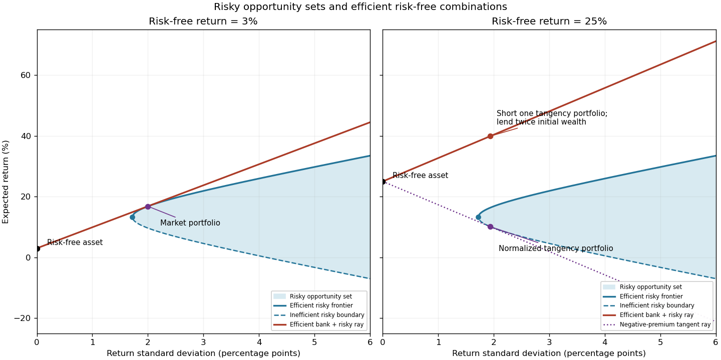
Risky opportunity sets and efficient risk-free portfolio combinations at risk-free returns of 3 and 25 percent
. Details. 
Write and let denote the risky holdings as fractions of total wealth. The remaining fraction is in the risk-free asset. Consequently their excess expected return is and their variance is . The Cauchy-Schwarz inequality in the inner product defined by givesEquality with positive excess return holds precisely for , , where . Thus solving determines both the efficient risky direction and the upper capital market line slope. Provided , the normalized market portfolio and its Sharpe ratio areHere the excess means are , so the required equations areThe leading principal minors of are , and , so Sylvester's criterion verifies positive definiteness and the solution is unique.
Direct substitution into the three equations givesSince the covariance matrix is invertible, this identifies its unique solution:The original PDF has all three components; the converted TeX's damaged binomial notation should not be used.
The risky weights of the normalized market portfolio must sum to one. Since , divide each component by this sum:Every weight is positive in this case, although the optimization permitted short selling.
The expected return of the market portfolio is the weighted mean of the asset returns:For its variance, use rather than expanding nine terms:Hence its return standard deviation isMeans and standard deviations here are both measured in percentage points, consistently with the given covariance matrix.
The excess expected return is . Dividing it by the return standard deviation yields the Sharpe ratio and upper capital market line slope:
All three individual risky assets now have negative excess expected returns. The covariance matrix and the risky portfolio opportunity set remain unchanged, but the risk-free point moves above all three individual means. Solving the new tangency equations givesThe sign of the normalized tangency portfolio now matters. Normalizing to a unit risky budget givesand its Sharpe ratio is . This point touches the lower risky frontier, rather than being an efficient positive-premium market portfolio.
The positive-premium efficient direction is still , . It shorts the first two assets, holds a hedging long position in the third, and has negative total risky investment. Its risk-free investment exceeds its initial wealth: the net proceeds of short selling are lent. Equivalently it takes a negative position in the normalized tangency portfolio. ThusNegative excess means therefore do not eliminate efficient risky investments when unrestricted short selling is allowed. The second diagram shows both orientations; it would be incorrect to interpret the negative normalized ratio as a negative slope for the upper efficient ray.
Indifference means equality of the risky expected utility and the utility of the sure reduced wealth. A second-order Taylor expansion, using , givesFor the sure alternative,Equating these and retaining the leading terms produces the small multiplicative risk premiumFor increasing concave utility functions this is positive. The approximation assumes genuinely small shocks with controlled Taylor remainders and positive final wealth; small variance alone would not justify it for rare large shocks.
Constant relative risk aversion coefficient means that does not depend on wealth, for and . The defining differential equation integrates asA second integration therefore givesThe additive constant and positive scale do not affect expected utility preferences. Since , positive gives risk aversion, zero gives risk neutrality, and negative gives risk seeking. These are respectively concave, affine and convex utility functions. The usual CRRA utility class is the positive- case.
Use for current wealth and for the dollar position in the risky asset. Its controlled dynamics have drift and diffusion coefficient . Over a short time step , the dynamic programming principle givesApply Itô formula to the second term, divide by , and let . The Hamilton-Jacobi-Bellman equation isFor the increasing concave value function, and , so the expression is a strictly concave quadratic in the risky position. Its derivative vanishes atSubstitution of this maximizer yieldsThere is a running utility reward but no consumption withdrawal in the wealth dynamics. The required concavity is also verified explicitly by the positive coefficient in part (d), so this stationary point really is the maximum.
The power-wealth investment with running utility objective is homogeneous of degree in wealth: scaling both wealth and positions by scales the reward by . Accordingly set . ThenFor completeness the remaining equation is , , whereThis confirms . The constant optimal risky fraction also makes wealth a positive geometric Brownian motion when started positive.
Financially the relative risk aversion coefficient is . Increasing reduces risk aversion, raises the risky fraction, and decreases the bond fraction: its derivative is . If the risky fraction is below one, some wealth is lent; at one, none is invested in bonds; above one, represents borrowing to leverage the risky position. As the risky fraction becomes unbounded, consistent with the absence of a finite unconstrained optimum for linear utility and positive excess drift. As the limiting fraction is , the logarithmic-utility allocation obtained by the appropriately rescaled power-utility limit; the literal objective at would be constant and would not select a unique strategy.
A process is a -martingale relative to the filtration when it is adapted, each is integrable, andHere adapted means is -measurable, and integrable means . Thus its present value is the conditional mean of its next value given all present information.
By the tower property of conditional expectation and the defining martingale identity,Iteration givesThe integrability in the definition ensures these expectations exist.
A previsible strategy selects using only , before the price changes from time to time occur. Thus these holdings cannot exploit future information.
The self-financing portfolio condition values both the old and newly rebalanced holdings at the same time- prices:Their equality says that rebalancing uses only the proceeds of selling existing assets: there is no external deposit or withdrawal. In particular, the changes in holdings have zero net cost at the current prices. The holdings for the following period may use the newly available information in .
At time , the self-financing portfolio can be valued using the holdings about to be carried over the next period:Subtracting this from gives the gains identityConversely, suppose the gains identity and the valuation hold. Rearranging the identity gives . Comparing with the valuation using shows that rebalancing at costs nothing. Applying this at each rebalancing time recovers the self-financing condition.
Assume the bank account stays positive and write and . Dividing the time- rebalancing equality by givesThe discounted bank account has constant price one. This is exactly the self-financing equality in the discounted market. Equivalently, subtract the corresponding valuation at to obtain the discounted wealth equation in discrete timeThis algebra uses only positivity of , and does not require it to be deterministic.
The usual replication argument needs two hypotheses implicit in the pricing conclusion: the strategy must replicate the payoff, , and its discounted gains must be integrable. Bounded predictable risky holdings suffice for the latter. Under these conditions, the equivalent martingale measure and part (c) giveThus discounted wealth is a martingale, and repeated conditioning givesFor a normalized initial bank account, , deterministic terminal bank value, and trivial initial information, this reduces to the intended risk-neutral pricing formulaIf is random it must remain inside the expectation. If a claim is not replicable, the existence of an equivalent martingale measure alone does not make its arbitrage-free price unique.
The discounted wealth martingale integrability condition cannot simply be dropped. For a concrete counterexample, set , , , and , where is uniform on and an independent fair sign. These positive bounded prices form a martingale in the natural filtration. Start with zero holdings; at time one buy shares financed by borrowing . This is previsible and self-financing, but its terminal wealth is , whose absolute expectation is infinite. It is therefore not a martingale. The stated pricing proof applies to the standard integrable replication class, rather than all unconstrained previsible strategies.
For an invertible continuous cumulative distribution function, monotonicity givesThus each transformed observation has the desired distribution. More generally use the quantile function ; the same event identity proves inverse transform sampling even when there are atoms. Independent uniform inputs give independent transformed samples; mere uniform marginal distributions do not imply independence between different samples.
One route is inverse transform sampling: if is the standard normal cumulative distribution function, then has the normal distribution with mean and variance .
Alternatively the Box-Muller transform uses two independent uniform inputs :To verify this, set and . The radial density is for , and the angle is independent and uniform. Their joint density is . Changing to Cartesian coordinates divides by the Jacobian determinant , givingThis factors into two standard normal densities, proving both normality and independence. Then provides the required means and variances. Implementations must avoid the zero input to the logarithm; ideal continuous uniforms hit it with probability zero.
Let denote the strike, , and suppose , , and . Under the Black-Scholes model and the risk-neutral measure, is normal withApplying risk-neutral valuation to the European call option payoff givesUse , whose differential is precisely the normal density times . The threshold is , soEquivalently, rescale the tail interval to obtain on .
For independent uniform inputs, the Monte Carlo estimator is . It is unbiased, converges by the strong law of large numbers, and has variance . The payoff has finite second moment because the lognormal stock has finite moments. Its estimated standard error is the sample standard deviation divided by .
Three useful methods are antithetic variates, a control variate, and stratified sampling. Their purpose is to reduce sampling variance at comparable computational cost, rather than merely to take more samples.
For antithetic variates, generate independent pairs and average both payoffs. Since the call integrand is increasing, the two values have nonpositive covariance. Indeed, for an independent copy , twice that covariance is the expectation of , which is nonpositive pointwise. With evaluations, the paired average has varianceFor a control variate, use the same simulated discounted stock value , whose known mean is . Replace the discounted call payoff by , preserving its mean. Minimizing its quadratic variance givesA predetermined coefficient or an independent pilot estimate preserves exact unbiasedness; fitting the coefficient from the same observations requires care.
For stratified sampling, divide into equal intervals, sample independently and uniformly within each, and average their payoffs. If is the conditional variance in interval , this unbiased estimator has variance . The law of total variance gives , so this is at most the variance of ordinary independent samples. Stratification removes randomness in how many samples fall in each region, which is particularly valuable when conditional payoff means vary strongly.
Take a unit-face zero-coupon bond with . Its continuously compounded zero-coupon yield to maturity, instantaneous forward rate, and short rate areThe last equality assumes the appropriate maturity differentiability at the diagonal. Integration of the forward-rate definition and differentiation of the yield definition giveAt fixed observation time , the yield curve plots this yield against maturity ; it describes today's discount prices at different horizons. Forward rates are extracted from these prices, not identified with the subsequent realized path of the short rate.
The common short-rate market price of risk follows from absence of arbitrage, with the securities driven by the same Brownian motion. Take two traded derivatives with drifts and diffusion coefficients . At a given state hold units of the first and of the second, and place in the bank account. The portfolio has zero current value and zero diffusion exposure. Its instantaneous excess drift isIf this were nonzero, selecting its positive orientation and maintaining the local risk-cancelling self-financing hedge would generate a gain without risk from zero wealth. Under the usual trading and regularity assumptions this violates absence of arbitrage. Thus the expression vanishes, and at nonzero exposuresAt zero exposure the correct relation is , without dividing by zero. This is a condition on traded securities: the physical drift of the nontraded short rate alone does not determine .
For sufficiently smooth, Itô formula under the physical measure givesHence and . Substitute these into the common risk-price condition from part (b), obtaining the Cox-Ross short-rate pricing equationFor a terminal payoff the final condition is . Writing prices as functions of requires the relevant Markov state to be sufficient for the claim; a path-dependent payoff generally requires additional state variables. The negative sign in is the adjustment from physical to risk-neutral rate drift.
The unit zero-coupon bond pays one at maturity. Its risk-neutral valuation therefore isNo particular rate coefficients were specified, so this expectation is the general answer; evaluating it further requires a chosen one-factor short-rate model.
For the alternative derivation let be the bank discount factor. For an integrable discounted payoff, pricing giveswhich is a martingale by the tower property of conditional expectation. For a payoff determined by the Markov rate state, this conditional expectation is represented by the indicated pricing function. A path-dependent claim requires an appropriately enlarged state, as in part (c). Now has finite variation. Applying Itô formula and the product rule under the risk-neutral measure, whose rate drift is , yieldsUnder the smoothness and integrability conditions used above, the martingale has zero finite-variation drift. The bracket therefore vanishes, giving againFor the bond the terminal condition is . This argument also shows why stochastic discounting remains inside the conditional expectation.
Articles by others on the same topic
There are currently no matching articles.