Let . For , the resulting compound Poisson distribution hasThus the merged claim size probability distribution is a rate-weighted mixture distribution, not an equally weighted mixture distribution unless the rates agree.
To prove this without any moment-generating function assumption, let be the characteristic function of a claim of type . Conditioning on its Poisson distribution count givesIndependence of the aggregate risks therefore givesThe weighted characteristic function inside is precisely that of the displayed mixture distribution. This is the transform of a sum of independent claims with independent count , proving the claim by uniqueness of characteristic functions. This is Poisson superposition of insurance portfolios. If , all risks make no claims almost surely and ; the severity law is then irrelevant.
Use the preceding construction with type- claims of deterministic size . For , the answer isThe characteristic function verifies this directly:Hence has the stated compound Poisson distribution. Distinctness of the makes the atomic probabilities unambiguous.
A zero coefficient is allowed. It corresponds to zero-sized claims in this representation and contributes nothing to . If a representation using only positive claims is preferred, remove that category: its count parameter becomes , with probabilities on the positive values. The zero claim sizes in a compound Poisson representation explain why the count parameter need not be unique. If , or if all positive-size categories have zero rate, the aggregate is identically zero.
Define . Grouping equal claim sizes gives the pathwise identityConditional on , the independent claims receive category labels with probabilities . There are assignments producing prescribed category counts, and every assignment has probability . Thus the conditional probability distribution is a multinomial distribution:when the nonnegative counts sum to , and is zero otherwise.
For , condition first on and use the probability generating function of a Poisson distribution:This factorization is the joint probability generating function of independent Poisson distribution variables. HenceA category with has zero count almost surely. The categorical thinning of a Poisson claim count produces independence after averaging over the random total, even though the counts are constrained to sum to conditional on that total.
Let . Conditioning on givesWhere the moment-generating function is finite around zero, differentiating the cumulant-generating function givesIn particular and . These compound Poisson cumulants use raw claim moments. The first two formulas also follow by conditioning: and , soThis is the law of total variance. They therefore remain valid with finite first two moments even when no positive exponential moment exists.
Under per-claim excess of loss reinsurance, put and let be the positive part of the excess. The insurer and reinsurer totals are sums of these payments over the same Poisson distribution count. Write . Using the tail integral formula for moments on the tail probabilities of and givesFor example, after , and shifting by gives the reinsurer formula. The moment formulas are finite whenever the corresponding claim moments are finite.
For the specified Pareto distribution, with shape three and minimum ,If , every claim exceeds the reinsurance retention. ThereforeIf , the tail integrals instead giveConsequently the requested sum of variances isOn the first branch, ; it decreases until and then increases. On the second branch . For the minimum is unique; if , all variances are zero and every reinsurance retention minimizes them. ThusThe curve starts at , reaches this minimum, passes through with matching slope on both branches, and then increases concavely toward the horizontal asymptote . The variance-minimizing retention for shape-three Pareto claims is shown below.
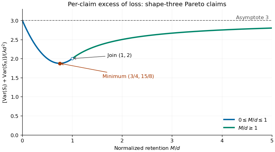
Sum of insurer and reinsurer aggregate variances for shape-three Pareto claims, minimized at retention three quarters of the minimum claim size
. Details. 
The two aggregate payouts are dependent. Conditioning on the common count gives covariance , so for every reinsurance retention, as required by . The covariance of two components of a compound Poisson sum accounts for this distinction between a sum of variances and the variance of a sum.
There is a moment domain qualification for this heavy-tailed example. For every , , and moments of order also diverge. Thus its positive moment-generating function is not finite and higher finite cumulants cannot be obtained by differentiating around zero. Its mean and variance calculations above are valid by conditioning or by the first two right derivatives at zero of the Laplace transform of a nonnegative random variable.
For nontrivial positive claim sizes in the classical risk model and , the adjustment coefficient is the unique positive solutionIndeed, has , , and is strictly convex. It becomes positive near the right endpoint of the moment-generating function domain. For a finite endpoint this follows from the assumed divergence; for an infinite endpoint, for some gives an exponential lower bound on , which eventually exceeds any linear function. Convexity gives existence and uniqueness of the positive crossing and .
Put and . Substituting into the supplied survival renewal equation for a classical risk model, and using , yieldsMultiplying by gives the proper renewal-type equationThe exponential tilt of the ruin renewal kernel turns a defective kernel into a probability density function, because the tail integration identity givesThis identity follows also by integrating and applying Tonelli theorem. The tilted probability density function defines a nonarithmetic distribution, even if the claim size probability distribution itself has atoms.
Differentiate to calculate its mean:It is finite and positive because is inside the finite moment-generating function domain. Next, reversing the order of integration givesThe forcing function is directly Riemann integrable. Choose with . Markov's inequality bounds by , so is bounded by a constant times . It is continuous; on finite intervals continuity controls its Riemann sums, and the exponential envelope controls the tails. These are sufficient conditions for direct Riemann integrability.
Iterating the renewal equation by convolution gives , where is the renewal measure. The remainder after iterations is bounded on each fixed interval by a constant times the chance that a sum of positive interarrivals remains in that interval, which tends to zero. The key renewal theorem, applicable to this nonarithmetic distribution of finite mean and the directly integrable forcing, now gives the interior adjustment coefficient ruin prefactor:Both numerator and denominator are positive, so .
For the unit-rate shape-two Erlang distribution, , and . Write , so positive loading requires . Dividing the adjustment coefficient equation by its nonzero root gives . ThusThe last simplification uses ; it is the Erlang shape-two ruin prefactor. Its value depends on the premium-to-arrival ratio, which is not specified numerically.
For the final exponential representation, evaluating at zero in the survival renewal equation for a classical risk model gives . If the slower term is present, necessarily and . Comparing with the finite positive asymptotic constant just proved yieldsA smaller adjustment coefficient would make the limit zero and a larger one would make it infinite. Here the leading exponential term determines a ruin adjustment coefficient. The coefficient need not be assumed positive to identify the leading term.
The wording does not specify that is nonzero. If and , the only surviving term instead gives , and . This case is realizable: claims with an exponential distribution of rate have ultimate ruin probability . Negative would make the ultimate ruin probability negative for large , and both coefficients zero are incompatible with a nontrivial positive claim rate and mean. These observations specify the coefficient qualification needed for the usual answer.
Use the shape-rate convention for the gamma distribution , with prior distribution probability density function proportional to . The observations are independent conditional on the common parameter . Unconditionally a common nondegenerate prior distribution induces covariance between distinct observations, so the Bayesian inference model requires conditional independence.
For unit-exposure counts, the likelihood is proportional to . Multiplying by the prior distribution givesThe future count has conditional expectation , so posterior distribution averaging givesThis is an exact Bayesian credibility estimate, with credibility factor and collective mean .
For the insurance exposure and claims inflation calculation put , assuming , and positive policy counts . Let be the total claim count in year . Conditional independence of the policy counts gives , and the observed average amount satisfiesFor possible observations, the recovered are nonnegative integers. If they are not, the data have zero likelihood under the model and no conditional posterior distribution is defined for those impossible values.
Write and . Since and determine each other, conditioning on the observed average amounts is equivalent to conditioning on these counts. The independent yearly count likelihood isThe Poisson-gamma conjugacy with unequal exposures therefore givesFor the future year, ; the number of future policies cancels because is a per-policy average. HencewithThe collective mean is the prior distribution expected claim amount per policy in the future year's monetary units. The experience mean first inflates each past per-policy amount to that same future year and then averages with policy-exposure weights. Equivalently, it estimates annual claim frequency by total observed claims divided by total past insurance exposure and converts that frequency to the future claim cost. This is inflation-adjusted Poisson-gamma credibility.
For fixed prior distribution parameters, increases strictly with total past insurance exposure: , and as . The prior distribution weight decreases to zero; acts as equivalent prior distribution insurance exposure. With no past insurance exposure the appropriate weight is zero and the prediction is , without defining an empirical experience mean.
Articles by others on the same topic
There are currently no matching articles.