For fixed, the denominator stays away from zero, so dominated convergence givesThis approximation remains appropriate on the left of the transition when . To resolve the Lorentzian peak approaching an integration endpoint, let with bounded , and put . The cosine is in the contributing region. ThereforeThus the distinguished transition has width . For large negative this expression matches to leading order; for large positive it gives the full interior-peak contribution.
For away from the transition, the denominator has a narrow minimum at . Set and . The slowly varying cosine may be frozen over the peak and the integration limits extended, givingThe small parameter controlling the left-end truncation near is , so this formula requires there.
For , the peak approaches , but its width is whereas its distance from that endpoint is . Their ratio is , and the relative variation of the cosine across the peak is also . Hence proximity to the endpoint does not destroy the approximation: the peak becomes narrower still. Equivalently, gives , with its peak at . The large- limit of the leading result is .
Take the usual Heaviside step function, for and for . Its Fourier transform must be interpreted as a tempered distribution. For , exponential damping gives an ordinary integral:Against any Schwartz function , the first term is an approximate identity of total mass : changing variables gives the limit . For the second term, pair positive and negative near zero. The difference removes the singularity and gives the Cauchy principal value of . The tails converge by dominated convergence. Since the damped functions also approach as tempered distributions, continuity of the Fourier transform yields the Fourier transform of the Heaviside step function:The printed plus sign is inconsistent with the printed convention for this . In fact requires ; the printed expression would give . Its plus sign would instead be correct for .
To find the Fourier transform of a principal-value reciprocal, exponential damping of its odd part givesThe integral vanishes at and its -derivative is , so it equals . Taking the distributional convergence limit givesAn ordinary improper integral of across zero is not a substitute for the specified Cauchy principal value.
The locally integrable function defines a tempered distribution. Its distributional derivative is : perform integration by parts outside , and observe that the boundary contribution tends to zero. By the Fourier transform of a derivative and the preceding result,Division by needs a finite-part inverse-absolute-value distribution, since is not locally integrable at zero. One possible normalization isIt satisfies . The general solution of is a multiple of the Dirac delta distribution: a test function vanishing at zero can be written , so depends only on its value at zero. Consequently the Fourier transform of the absolute logarithm isChanging the finite-part normalization changes . The printed reciprocal expression is meaningful with this interpretation, not as an ordinary function at .
The barred integral in the PDF denotes a Cauchy principal value. With its left side is the convolution , whose Fourier transform is . The right side is on and zero outside; either direct integration or the Fourier transform shift rule givesThus, away from the irrelevant single point in the formulation,By the Fourier transform of the absolute logarithm, the difference has transform ; its two delta terms cancel. ThereforeIts endpoint logarithms are locally square integrable, and at infinity, so it belongs to L2 space. The Hilbert transform multiplier is invertible almost everywhere on this space, proving uniqueness there. Without a decay or function-space condition, one may also add a constant under the symmetric principal-value convention. If the reversed step function were used to retain the printed sign in part (i), this answer would acquire the opposite sign.
Write locally, with analytic and . The coefficient of in the Modified Bessel differential equation requires . If , its recurrence is , with . HenceThe analytic part is even: an odd-power term in would produce an uncancelled odd-power term under the same differential operator, and the recurrence removes all such terms. Insert a smooth even cutoff equal to one near zero. The smooth part and the exponentially decaying tails give no algebraic large-wavenumber terms after repeated integration by parts. Therefore the logarithmic singularities determine the requested terms. For ,Thus the Fourier transform of the modified Bessel function K0 has expansionAn independent check follows from the integral representation of the modified Bessel function of the second kind. Integrating first and then setting gives , with exactly these first two terms.
Use the Gaussian pole transition for a large gamma parameter. With and , Taylor expansion givesThe upper semicircle is traversed from left to right, so on the indentation. The minus sign in therefore makes its contribution . The remaining leading integral isAt its Cauchy principal value vanishes by oddness. Differentiating with respect to removes the pole, leaving the Fourier transform of a Gaussian:Integrating from zero givesThis is uniform for bounded real (and extends analytically over bounded complex values where the local contour is continued consistently). Contributions away from the saddle are exponentially small after localization. The bounded shift enters at the next order, not the leading error function. For example, retaining the displayed cubic correction gives as the next term. This also checks the constant and contour sign.
For positive integer and any positive integer , the finite geometric series identitygives an exact decomposition along the indented contour. The polynomial terms have no pole and may be returned to the positive real axis; their Gamma function integrals areEquivalently, expansion about the endpoint in the Laplace transform integral gives the same coefficients. The resulting formal asymptotic expansion isThe ratio of consecutive terms is , so the infinite series is factorially divergent. It should be truncated, not treated as a convergent sum; the pole prescription controls the contribution beyond its algebraic orders. Although the source initially calls an integer, the ordinary lower endpoint integral requires , as is already implicit in the large-positive- limit of part (i).
By Stirling's approximation, for fixed ,Apply this with and use . Their exponents add to one, and henceMore explicitly, the ratio is . The exact ratio of neighboring terms isThus the Airy function expansion is factorially divergent, and optimal truncation retains about terms.
The printed summation starts at , but its leading term is missing. The Gamma reflection formula gives , so . The correctly normalized dominant Airy function expansion starts at zero. This correction is essential for the exponentially small remainder in the next part; if the printed series is used literally, its remainder also contains the entire missing leading term.
Let , choose a consistent branch, and truncate the corrected series after , with . The leading factorial tail in part (iii) is represented by the same indented integral as in part (ii):Here the divergent sum means its lateral Borel summation, not ordinary summation. To see why the pole approximation controls this remainder, write and insert in the leading late terms. Summing the geometric tail creates ; produces . The relative corrections to the late coefficients give lower-order contributions on its saddle scale. More concretely, the Borel transform of the coefficient series isThe simple pole supplies the leading Stokes phenomenon; its weaker logarithmic singularity supplies the smaller corrections. This is the integral justification for retaining the factorial tail.
For , expand . Part (i), with , now givesThis formula uses the upper-pole prescription and the upper Airy function switching ray: near , take near zero. The coefficient of the subdominant exponential changes smoothly from zero to across this ray and has value on it. The angular transition width is . The conjugate lower ray has the conjugate contour sign, rather than the same on both rays. This is error-function smoothing of a Stokes multiplier, not a discontinuity of the analytic Airy function. With the literal printed series, the missing would invalidate this remainder formula.
The outer solution satisfies , so on a connected interior interval the nonoscillatory branches are and . Both happen to solve the differential equation exactly away from any endpoint mismatch. For a fixed positive endpoint coordinate ( or ), introduce the inward distance on the left or on the right. The leading nonlinear endpoint layer with a quadratic reaction obeysMatching to zero fixes , so . It is negative for every sufficiently small nonzero . Thus no real nonconstant layer can approach zero: the zero outer branch requires , and then is an exact solution.
Matching to fixes . The first integral factors asConsequently an endpoint value can match this branch only if . For , there are two choices: a direct approach to , and an initial excursion to followed by a return to . Both are translations ofThe negative translation gives the direct layer; the positive translation gives the excursion. At the two coincide, with the maximum at the wall. For , the unique admissible direction is a monotone approach from below:where is fixed by . At only the constant leading layer matches at a finite inward coordinate; a pulse translated infinitely far from the wall is outside this endpoint-layer classification.
Thus the leading admissibility condition for the negative outer branch is and . Under strict inequalities, each endpoint has two choices when its datum lies between and , and one choice below . Their independent combinations give one, two or four formal matched profiles. In particular, for there are four negative-bulk profiles in addition to the exact zero solution, so uniqueness certainly cannot be inferred from the outer equation. The endpoint equalities and the constant-layer cases are degenerate; higher-order endpoint matching is needed to decide exact finite- counts at these cutoffs. These conditions and counts concern leading families under the stated exclusion of interior layers and rapid oscillations.
A matched asymptotic expansion for the negative branch isThe following sketch shows the four choices for zero endpoint data, together with the exact zero solution. It plots leading composite profiles, not numerical claims of exact finite- multiplicity.
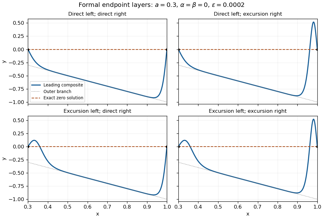
Four leading endpoint-layer profiles with negative outer branch, and the exact zero solution
. Details. 
Additional interior layers cannot be excluded merely by counting the outer roots. Freezing gives a homoclinic orbit to with the same hyperbolic-secant pulse. Its location would require a further matching or solvability condition; it is not an arbitrary parameter in the original variable-coefficient problem. Indeed, put . The exact equation and an energy identity areAn isolated order-one pulse with exponentially small tails on both sides would decrease this energy by an algebraic amount, whereas its two tail energies would be exponentially small. This obstructs a freely standing isolated pulse well away from the walls. It does not by itself classify oscillatory solutions or pulse interactions with endpoint layers, so a complete global uniqueness claim would exceed this leading construction.
When , the two outer roots meet at the left endpoint. Let , . Balancing with gives , and balancing with them gives . The one-third-power scaling at a nonlinear turning endpoint is thereforeIts left condition is . Matching to the negative branch requires and as ; the right endpoint is then handled by the earlier layer. Write . In the intermediate matching region a small correction satisfies , so . The growing Airy function excludes ; the decaying Airy function supplies a permissible stable matching direction. In fact is an exact inner solution satisfying , establishing existence of an inner match without solving a nonlinear shooting problem. Since , the wall condition excludes an infinitesimal nonzero decaying correction about this solution; it does not prove absence of other finite-amplitude inner solutions. The right wall still requires at leading order.
Matching instead to zero requires . Its linearized equation is , with solutions and . Their large- forms have envelope and phase ; although their values decay, they generate rapid spatial oscillations in the overlap region. The imposed nonoscillatory assumption removes these nonzero tails. The exact remains, and a globally zero outer branch again requires . The PDF's integration hint uses an inverse hyperbolic tangent; the converted TeX's inverse tangent would give a different and incorrect primitive.
Put and use the method of multiple scales with . At leading order, , so write with , . The order- equation isUsing , its fundamental sine coefficient is , and its fundamental cosine coefficient forces . Removing these resonant forcings is the solvability condition in the method of multiple scales. Thus the shifted Van der Pol amplitude evolution isWith and , solve by putting . This givesThe uniformly valid leading approximation is on bounded slow-time intervals for which remains bounded. The exact initial derivative is recovered by the first-order correction; the displayed leading expression already satisfies the leading initial data.
There is an important limitation to the source's unqualified time-range wording. Starting from , the amplitude decays for , is constant at leading order for , and grows for . In the latter case the denominator vanishes atA bounded-amplitude multiple-scale expansion is uniform for , not through its predicted large-amplitude breakdown. For the decaying case every fixed bounded slow-time interval is available; the leading unstable equilibrium at also has bounded amplitude over such intervals. The envelope singularity is a breakdown warning, not a proof that the exact original solution has precisely this blow-up time. The coefficient in the PDF is , correcting the converted TeX's duplicated .
Again put . To leading order the oscillator has form , while the second variable has a slow part . Averaging its equation over the fast period givesThe oscillatory forcing of the second variable produces only an order- correction: its leading fast derivative is , whose bounded primitive is . Thus it creates no secular term.
The oscillator solvability condition is the same as in part (i), with replaced by :Introduce accumulated slow timeThe shifted Van der Pol amplitude evolution therefore gives, for ,ConsequentlyAs before, uniformity for means a fixed bounded slow-time interval on which the envelope stays bounded. For it fails when reaches , with limiting value at . There is no bounded leading approximation covering all such slow times for arbitrary positive .
Use the Burgers reduction of weakly nonlinear rightgoing acoustics, with , , and . The equation of state expands asAt order one, mass conservation and momentum conservation give and . For the pure rightgoing acoustic wave with no independent leading mean density or velocity shift, . This is the background choice implicit in the requested traveling-wave expansion; additional mean components would modify its phase convention. The source's duplicated phrase about expanding should refer to expanding as well as .
At order , the mass conservation equation becomeswhereas the momentum conservation equation becomesIn the latter equation, the two nonlinear products and cancel. Substitute the equation of state relation into the former equation and add the two equations to eliminate the first corrections. The result isThe same calculation gives , so the first corrections may be chosen without an explicit secular factor of . This is why the retarded-time description can remain uniform for , provided the leading profile and its relevant derivatives remain bounded over that range and the slow propagation interval.
This Inviscid Burgers equation can develop a shock, so the source's uniformity assertion needs a pre-shock qualification. If and , its method of characteristics givesThe smooth construction ends when this denominator vanishes; if , the first such distance is .
For viscosity write with bounded positive . Since , the order- momentum conservation equation instead reads . Addition now yields the viscous Burgers equationIts positive diffusion resolves the inviscid steepening rather than supporting an unqualified smooth inviscid expansion through shock formation.
Assume , the positive diffusivity requirement for the forward heat kernel. A normal mode of the linear complex Ginzburg-Landau equation givesFor real , the maximum temporal growth rate is . The Briggs-Bers criterion starts the inverse time Laplace transform above the temporal growth spectrum and follows the two spatial roots as its frequency contour is lowered. A contributing spatial pinch point occurs when roots continued from opposite sides of the spatial contour coalesce and prevent its deformation. An arbitrary algebraic saddle is not sufficient without this branch selection.
Here givesTo check the pinch, start at with large. The roots are and initially lie in opposite half-planes. They meet at , giving the causal saddle. Positive imaginary absolute frequency means fixed-position exponential growth. ThereforeFor there is no positive temporal growth. At the fixed-position exponential rate is zero; its algebraic prefactor, derived below, decays. When the convective interval is empty.
The source specifies only real coefficients. For , temporal growth is unbounded at high real wavenumber, so the usual causal forward-diffusion construction is ill posed and the above criterion does not apply. For the equation reduces to transport with amplification; its point impulse remains a moving delta, rather than a spreading heat kernel. These cases cannot be included by division by .
Select the causal Green function, zero for ; otherwise the impulse equation permits arbitrary homogeneous additions. Use the spatial Fourier transform convention and the temporal Laplace transform boundary convention . The transformed impulse equation isIf , a literal real-frequency Fourier transform of the growing response need not exist. Its causal inverse instead starts on and is continued from there. For close the frequency contour below; its clockwise orientation and the pole residue give . For the upper closure contains no pole. The remaining inverse spatial transform is a Gaussian integral:The unit-mass Gaussian heat kernel tends to at , giving the required impulse normalization.
At the advected center , its amplitude is . At a fixed spatial point,Thus permits growth of the moving wave packet, but it is convective hydrodynamic instability if the fixed-position rate is negative. A positive fixed-position rate is absolute hydrodynamic instability. At its equality threshold the factor decays, explaining the marginal exponential classification. This directly verifies the physically selected Briggs-Bers criterion saddle rather than assuming its accessibility.
Write and . A well-posed anisotropic diffusion problem requires to be symmetric positive definite: and . For the normal mode in the source the dispersion relation isThe group velocity vanishes when . ConsequentlyThe requested anisotropic absolute-instability threshold for positive diffusion isFor positive definite diffusion this is also sufficient: the anisotropic Gaussian heat kernel has exponential factor and a prefactor, so its fixed-position growth rate is precisely .
Let the prescribed speed be and let be the positive eigenvalues of . The Rayleigh quotient for givesAbsence of absolute hydrodynamic instability for every direction therefore requiresThis is an upper bound on , not a minimum required value. The source's last sentence reverses this monotonicity: reducing the growth parameter always helps, so there is no finite lower threshold guaranteeing absence. If it had asked for instability in every direction, the corresponding condition would be . Without the positive-definite assumption, negative diffusion directions make the forward problem ill posed; a singular diffusion tensor requires a separate transport analysis and does not support the displayed inverse-matrix formula.
Assume again positive diffusion . Remove the drift with . Differentiating explicitly cancels the first derivative and givesBalance the second derivative with the linear confinement by taking , so the requested exponent is . More precisely, putThe eigenvalue problem reduces to . Its two solutions are Airy functions. The growing is excluded by the condition at infinity: its growth proportional to dominates any linear-in- drift factor. The decaying remains admissible even after multiplication by . The wall imposes , so , giving the Airy global modes of a linearly confined Ginzburg-Landau equation:The least negative zero, , gives the largest temporal growth rate. HenceAt equality the leading global eigenmode is neutral, and below it all these eigenmodes decay. In contrast, freezing the coefficients locally gives absolute hydrodynamic instability wherever . Such a pocket exists iff and extends to . Thus global instability implies a locally absolutely unstable pocket, while the converse fails: a pocket shorter than does not overcome the wall and confinement losses. The additional threshold is order , precisely the loss produced by the Airy function spatial scale.
Articles by others on the same topic
There are currently no matching articles.