For a scalar, the Lie derivative of a function is its directional derivative:The Lie derivative of a vector field is their Lie bracket of vector fields:For a torsion-free connection,The last term vanishes because the connection coefficients are symmetric in . This proves .
For the metric tensor statements use the Levi-Civita connection, which also has metric compatibility. The tensor derivation property of the Lie derivative of a tensor field givesExpanding the first term using and using the vector identity cancels the derivatives of and . What remains isSince are arbitrary, the Killing equation isMetric compatibility is needed here, even though symmetry alone sufficed for the vector identity. In general the Lie derivative of a metric with nonmetricity contains a term . For example, with the metric tensor , zero connection coefficients and , the Lie derivative of a tensor field is , whereas . The usual metric connection interpretation of the question supplies the required compatibility.
For the Riemann curvature tensor calculation, keep the original PDF's convention. With and , it meansThus the commutator on a covector has the opposite sign. Write . Taking a covariant derivative of the Killing equation makes antisymmetric in its first two indices, while the Ricci identity givesCombining this with the first-two-index antisymmetry gives the three relationsAdd the first and third and subtract the second. Pair symmetry and the first Bianchi identity imply . ConsequentlyThis is the second covariant derivative of a Killing vector in the paper's convention; its sign is tied to the declared curvature-sign convention in Killing derivative identities, not to raising a particular index.
Set . Along any smooth curve with tangent vector , the chain rule and the just-proved identity give the Killing transport equationsChoose a parallel-propagated orthonormal frame along the curve. These become a homogeneous linear system of ordinary differential equations for the components of . Uniqueness of its initial value problem implies that zero initial data remain zero. Any point in the same connected component as can be joined to by a piecewise smooth curve. Therefore zero value and zero first derivative at force the Killing field and its derivative to vanish throughout that component, with no completeness assumption. On a manifold with one connected component this is the requested global result. Connectedness cannot be dropped: on two disjoint flat spacetimes, take the zero field on one and a nonzero translation on the other.
On a pseudo-Riemannian manifold of dimension with one connected component, the map is therefore injective. There are independent components of the value and of its antisymmetric derivative. The dimension bound for Killing vector fields isIt is attained in flat space by with constant antisymmetric , giving translations and infinitesimal rotations or Lorentz transformations. The four-dimensional maximum is 10. For a disconnected manifold the bound applies componentwise; there is no uniform global bound depending only on if the number of components is unrestricted.
General relativity models spacetime by a smooth four-dimensional Lorentzian manifold whose metric tensor governs clock readings, causal cones and free-particle motion. The Einstein equivalence principle motivates local special relativity and universal geodesic free fall for test bodies; it does not by itself select a unique gravitational field equation. We assume a Levi-Civita connection, a metric tensor as the gravitational field with no additional dynamical gravitational variables, and matter with a covariantly conserved stress-energy tensor. Units have .
The existence of local inertial frames is a local statement. At any regular event choose an orthonormal frame and Riemann normal coordinates, so that and at the event, with metric signature . Metric compatibility then gives there. The geodesic equation at that point is the special-relativistic inertial equation. Along a timelike geodesic, a parallel-transported orthonormal frame gives Fermi normal coordinates, eliminating the connection along the central worldline. These constructions do not in general eliminate second derivatives of the metric tensor in a neighborhood. The Riemann curvature tensor is built from the derivatives of the connection coefficients as well as their quadratic terms; nonzero Riemann curvature tensor components can remain when all connection coefficients vanish at a chosen point. Conversely, Polar coordinates in Minkowski spacetime can have nonzero connection coefficients but zero Riemann curvature tensor. Connection coefficients alone are therefore not an invariant measure of gravity.
For the tensorial content, consider a two-parameter family of geodesics parametrized by an affine parameter, with tangent and connecting field . Their coordinate construction gives , and torsion-freeness gives . Since , commuting derivatives in the convention of Question 1 yields geodesic deviation:The left side is covariant relative acceleration, rather than the second coordinate derivative of an arbitrary separation. In an orthonormal frame in free fall with , its spatial components are . This is a measurable tidal force, and a coordinate transformation cannot make a nonzero Riemann curvature tensor disappear. It is the distinction between gravity at one event and the behavior of an extended freely falling laboratory.
In a static Newtonian limit, and , so the test-body acceleration is . The curvature-sign convention in Killing derivative identities gives . Hence relative acceleration is the negative Hessian of the gravitational potential. For the Newtonian potential of a point mass , the Hessian has radial eigenvalue and two tangential eigenvalues : radial separations stretch and tangential ones compress. Outside the source the Ricci tensor can vanish while the Riemann curvature tensor remains nonzero. Its vacuum tidal part is encoded by the Weyl tensor; vacuum does not mean flatness. Gravitational waves likewise carry Riemann curvature tensor disturbances without a local material source.
To obtain the field equations, make the additional dynamical assumptions explicit: locality and diffeomorphism invariance of general relativity; a symmetric metric tensor field equation using at most second derivatives of the metric tensor; a geometrical left-hand side linear in the Riemann curvature tensor with constant coefficients; and compatibility with local matter conservation. These restrictions exclude higher-curvature or extra-field alternatives. Under them the available rank-two curvature contractions give the ansatzThe contracted Bianchi identity and metric compatibility giveFor this to vanish identically for arbitrary metric tensors, . Assuming and absorbing its normalization into the coupling givesThe permitted constant term is the cosmological constant. Its value is not fixed by the equivalence principle. Conservation of follows for generally covariant matter on its equations of motion: varying the matter action under a compactly supported infinitesimal diffeomorphism, then integrating its term by parts, gives . The divergence-free Einstein tensor is consistent with this identity.
The coupling sign must be fixed in the actual curvature-sign convention in Killing derivative identities, with . For the static weak-field approximation, . Set for the local asymptotically flat Newtonian comparison. In four dimensions the trace equation gives , so for slowly moving matter. Matching forces . Thus, with this convention,Under the opposite curvature-sign convention in Killing derivative identities the coupling sign reverses, as in Einstein-equation coupling under reversed curvature. This sign statement is compatible with the supplied linearized handout. Local inertial frames remove the connection at an event; tidal Riemann curvature tensor effects remain tensorial, and the field equations require dynamical assumptions beyond the equivalence principle.
For the static nonrotating source, use spherical symmetry and the static scalar perturbation of Minkowski spacetime, with isotropic radius :To first order, the Einstein tensor in the declared convention hasThese are also the static scalar perturbation of Minkowski spacetime equations in the original information sheet. The source has and zero spatial stress. With the sign established in Question 2,The distributional identity and asymptotic flatness give . For , the spatial field equation has trace and therefore . Its decaying spherical solution is , so . This determines both potentials; the spatial correction cannot be inferred from the Newtonian gravitational potential alone.
Now use the isotropic-to-areal weak-field radius change. The angular coefficient defines , hence to first order. Thus to the same accuracy, and replacing by inside a perturbation changes only second-order terms. With the Schwarzschild radius , the linearized Schwarzschild metric isThis is an exterior weak-field approximation: . The point source is used distributionally to fix the mass, not to claim a regular or weak field at the origin.
For a null geodesic choose its orbital plane as , using rotational symmetry, and let a dot denote an affine parameter derivative. For a Killing vector and an affinely parametrized geodesic tangent , the geodesic conserved quantity from a Killing vector follows directly fromApplying this to the time-translation and axial Killing vectors, with the spatial sign absorbed into the definition of , givesIf the tangent is normalized as the photon's four-momentum, is its energy measured at infinity and its signed angular momentum about the selected axis. Rescaling an arbitrary affine parameter rescales both; the ratio is the invariant impact parameter. Future-directed orbits have . Assume to use as the orbit parameter; gives radial rays, not a finite-radius circular orbit.
The null vector constraint givesExpand consistently to first order in the weak-field approximation correction: and . Also . Therefore the first-order orbital equation isThe cubic term is the first correction relative to the flat inverse-radius term; the equation is not a controlled exact equation for large .
A constant solution of a first integral is not by itself sufficient to establish a circular geodesic. For a circular trajectory, the radial Euler-Lagrange equation also requires , where now is the metric's time coefficient. Combining this with the null vector constraint gives , or . Equivalently, the formal potential must have a stationary point. Apart from the infinite-radius endpoint , its only stationary point is , with . Thus the formal circular solution requiresThe reduced radial equation is , with prime denoting . It follows by differentiating the first integral on moving segments and agrees with the regular Euler-Lagrange equation at turning points. Perturbing givesThere is an exponentially growing linear instability mode; equivalently . The formal circular orbit is unstable.
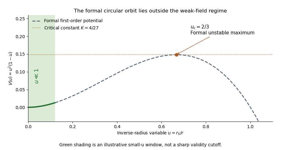

The weak-field photon-orbit validity limitation is essential: is not small. There is therefore no finite-radius circular photon orbit established within the controlled weak-field region. The formal extrapolation happens to reproduce the radius and impact parameter of the exact Schwarzschild photon sphere, but that physical result needs the exact geometry. The calculation also cannot establish a Schwarzschild event horizon from a first-order expansion at .
The physical spherical coordinates cover , , , and with periodic identification. The center and the polar axes are the usual coordinate singularities, rather than physical curvature singularities; a regular polar chart restricts and . For the null coordinates,Thus the physical metric tensor isThe conformal transformation followed by , gives , , andConsequently . Finally , converts to , yieldingThe ranges must retain their joint constraints:Equivalently, and , with . The angles retain their original ranges and identifications. Extending to negative values would double-count the radial polar geometry. The conformal factor isThe unphysical metric tensor extends onto the Einstein static universe, while physical Minkowski spacetime occupies the triangular region in its radial Penrose diagram. The edge is the regular center and belongs to the physical region away from its endpoints.
The conformal boundary consists of the following infinities. Future null infinity has , hence with , and corresponds to finite with . Past null infinity has , hence , and corresponds to finite with . Future timelike infinity is , past timelike infinity is , and spacelike infinity is . Although angles label points on null infinity, their two-spheres collapse at these three endpoint locations in the compactified picture.
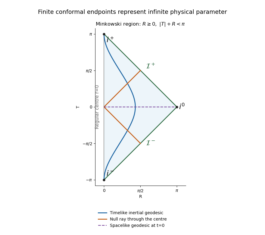
The radial Minkowski conformal diagram and the endpoints of timelike, null and spacelike geodesics
. Details. 
For the geodesic endpoints in Minkowski conformal compactification, one can check the limits directly. A timelike inertial trajectory is with . At both and tend to , so and the trajectory ends at future timelike infinity. At both tend to , giving past timelike infinity. This includes a stationary inertial worldline with bounded .
For a null inertial trajectory, . As , , so has a finite limit while ; its future endpoint lies on future null infinity. As , , giving a finite limiting and , hence a past endpoint on past null infinity. Radial null geodesic paths have constant. A ray passing through the center changes its angular direction; in the angle-suppressed radial diagram it reflects at rather than terminating there.
A spacelike geodesic is also a straight line, now parametrized so that . At either end, asymptotically, , , and the endpoint is spacelike infinity. A radial spacelike line at has two opposite-angle halves which project onto the same horizontal interval in the diagram.
The conformal compactification endpoints occur at finite but at infinite physical proper time or affine parameter; Minkowski spacetime is geodesically complete. The conformal preservation of null geodesic paths does not preserve an affine parameter: if is physically affine, an unphysical affine parameter satisfies up to a constant. Along a complete null ray this can have a finite integral at infinity. Timelike and spacelike physical geodesic paths are not generally geodesics of the rescaled metric tensor, so their drawn curves must not be interpreted as freely falling unphysical observers.
Finally, every physical event can send an outgoing null ray to future null infinity, so is all of Minkowski spacetime. Its black-hole region and intrinsic event horizon are empty. The null edges in the diagram are infinity, not horizons concealing part of the physical manifold. Complete inertial observers likewise have no observer event horizon. Accelerated observers restricted to a Rindler wedge can have a Rindler horizon, but that is observer-dependent and does not contradict the horizon-free Minkowski spacetime. The conformal diagram compactifies infinity; it does not introduce a physical horizon.
Articles by others on the same topic
There are currently no matching articles.