Substitution into the Newell–Whitehead–Segel equation gives . Thus a nonzero roll has ; at equality the branch meets the zero solution. The two signs of differ by a constant phase modulation.
The sign of the transverse zigzag instability must be calculated from the differential operator. Put and . The chain rule givesConsequently the change in the printed functional density isFor a Lyapunov functional one integrates this density over the transverse coordinate too, or uses a transverse spatial average, with periodic or decaying boundary conditions. A fast- average alone leaves a density depending on and is not itself a global monotonicity statement. Indeed under these boundary conditions, and the functional derivative of the resulting spatial integral is . Hence : stable rolls locally maximize this functional.
With the plus sign actually printed in , makes both quadratic contributions to negative. These rolls are stable to long-wave transverse phase modulation. For a sufficiently long-wave displacement increases and is unstable. At the second-derivative stiffness vanishes, but the fourth-derivative and nonlinear tilt terms still decrease . Linearization makes the conclusion explicit:Thus for the unstable band is , with maximum growth at ; in a finite periodic cell the band must contain an allowed Fourier mode. Replacing by reverses the sign of the detuning associated with the zigzag instability. It would therefore be incorrect to import that opposite sign convention into the printed equation. Transverse stability does not exclude the distinct longitudinal Eckhaus instability.
A uniform spatial translation of the rolls changes by a constant, so a local phase modulation equation cannot depend on itself. Reflection across the transverse axis acts as ; reflection across the roll coordinate acts as , after choosing a reflection-symmetric roll profile. The right-hand side must therefore be odd in and even under reflection.
At the lowest orders, and have these symmetries. The terms , and are even in and are forbidden; is odd under reflection and is forbidden. The first nonlinear derivative term at this order is . Near the transverse threshold use the quartic-time transverse phase scaling: the small coefficient of , the fourth derivative and this cubic term have the same asymptotic order. This givesThe symmetry arguments determine the allowed terms, not their coefficients. A well-posed short-wave regularization requires . The zigzag instability occurs for , since a Fourier mode grows at . With , differentiating givesFor the preferred uniform slopes satisfy ; their slope diffusion coefficient is . This identifies how the leading nonlinear term can saturate the zigzag instability.
Use the translation-covariant phase expansion with , and . Write all fast profiles at , including the corrections. LetThe Swift–Hohenberg equation has steady equation , and differentiation gives . On a fast periodic cell is a self-adjoint operator. We assume the translation mode is its only zero mode; otherwise one must impose the corresponding additional Fredholm solvability conditions and retain additional amplitudes.
Since , its squared operator is . The time derivative first contributes at order . At order ,The Fredholm solvability condition is orthogonality of this forcing to . Periodic integration by parts givesThus the condition is . General slowly curved rolls require at leading order. If , this order- residual first enters the order- equation, so the leading order- problem is solvable. In particular,is precisely the near-threshold condition. Defining and keeps the residual as the phase-diffusion term at the next order.
There is an important chain rule qualification in this part. The printed value of follows from the expansion. Its printed value of follows only if transverse differentiation of the translated correction profiles is omitted. For a consistent translation-covariant phase expansion, that omission is generally nonzero.
At the leading transverse threshold letwhere the last conditions fix the phase gauge. Put , , and , and use . At order the Fredholm solvability condition givesThe first two contributions follow directly by differentiating:Choose the reflection-symmetric roll with even. Then is odd and even. Projection onto the odd translation mode eliminates , and , leaving exactly the symmetry-allowed phase modulation equation. Its coefficients areandIf one freezes at the unshifted coordinate when taking transverse derivatives, , and its projection contributes only the term. The other two projected terms then give the printed expression . But freezing these profiles is inconsistent with the translated in for a general finite phase displacement. The printed expression needs the extra assumption , which is not an identity.
A small-amplitude calculation demonstrates the difference. For a critical roll of leading amplitude and fast wavenumber , the steady equation and giveThe third harmonic coefficient in follows by dividing its cubic forcing by the fast eigenvalue . Substituting in gives the displayed correction profiles; the near-zero first-harmonic eigenvalue in the even problem must be retained to obtain the first harmonic of . Periodic orthogonality then givesThus the supplied nonlinear coefficient is not generally an exact consequence of the finite-amplitude translated-roll expansion. The corrected coefficient above, the printed calculation under its additional freezing assumption, and the genuine near-threshold phase modulation equation are all distinguished explicitly.
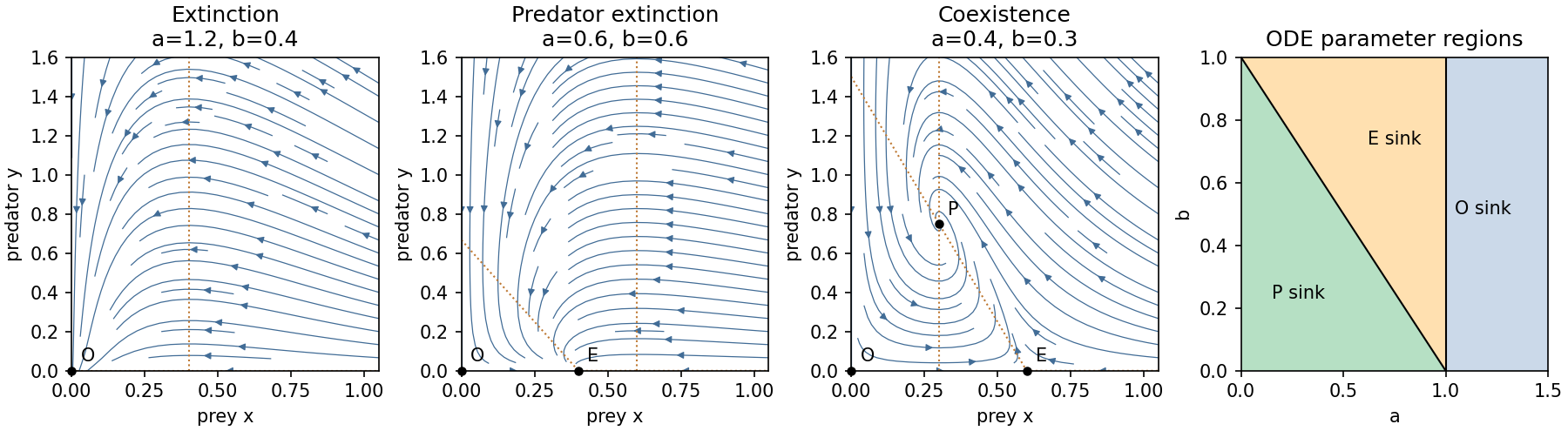
Write . The admissible equilibrium points are , when , and when . The Jacobian matrix isAt the eigenvalues are and ; at they are and . At a positive coexistence equilibrium point,It is therefore asymptotically stable. It is a node for , a focus for the reverse inequality, and has repeated real eigenvalues at equality. The node–focus change does not alter the attracting equilibrium point's topology.
There are three open physical parameter regions:
The axes are invariant. On , decays exponentially; on , prey obey the logistic differential equation. Positivity follows because each right-hand side has its population as a factor. Also is bounded by logistic comparison, while satisfies , so all forward trajectories are bounded. The Dulac function has divergence in the interior, excluding periodic orbits by the Bendixson-Dulac criterion.
In the extinction region, , and then is eventually negative. In the prey-only region, the upper bound implies predator decay and convergence of interior prey to . In the coexistence region the Lyapunov functionhas . Its positive-quadrant sublevel sets are compact, and the only invariant subset with also has . The LaSalle invariance principle proves convergence of every interior trajectory to . These facts justify the complete qualitative phase portraits, not just their local arrows.
At , and meet in a transcritical bifurcation; positive prey decay algebraically. At with , and exchange stability. On its centre manifold, gives , so the physically positive side is still attracting. There is no interior Hopf bifurcation since the coexistence trace never vanishes.
The characteristic polynomial of a real matrix is . Thus vanishes exactly when , and vanishes exactly when . These are the required eigenvalue conditions.
For and , the discriminant is negative, andTheir moduli equal one. Taking with gives . The strict trace inequalities exclude and hence exclude the repeated real multipliers .
The quadratic discrete predator-prey map equals the identity plus the vector field of part (a), so its admissible fixed points are the same . Their Jacobian matrices are the identity plus the corresponding continuous-time Jacobian matrices, but map stability requires eigenvalues inside the unit circle rather than the left half-plane.
At the multipliers are : it is a sink for and a saddle for . At they are and . ThereforeFor , the prey multiplier is below : is a saddle when and a repeller when . For , makes it a saddle. The crossings at and are the two transcritical bifurcations already encountered. The crossing at is a prey period-doubling bifurcation.
At positive coexistence,For clarity, derive the relevant Schur stability criterion directly: setting in givesThe open unit disk maps to . A real quadratic has both roots there precisely when all three displayed coefficients have the same positive sign. Since , the coexistence fixed point is a sink precisely whenThis region exists only for . In the coexistence triangle , put . If , one root lies below and the other in , so is a saddle. If but , it is a repeller; if , it is a sink. These signs give the complete local fixed-point partition, including real and complex multipliers.
The coexistence period-doubling bifurcation lies at ; its segment adjoining the sink region has . The other multiplier there is and lies strictly inside the unit circle on this segment. This coexistence flip is subcritical on that segment. To calculate its direction, normalize the eigenvector by and the left eigenvector by . The symmetric quadratic derivative is given explicitly in part (d). Eliminating the quadratic term from the one-dimensional centre manifold map gives the effective cubic flip coefficientFor a scalar reduced map , its second iterate satisfies . Thus on the stable-fixed-point side , and the two-cycle multiplier is . An unstable coexistence two-cycle meets the stable fixed point as increases to the flip curve. The other multiplier remains inside the unit circle. The complex unit-modulus crossing lies at , with . The two curves meet at with a double multiplier . The prey flip and predator invasion curves meet at with multipliers .
The sketches mark the sink regions and all these local thresholds. They are a local atlas, not a claim that the map has only these global attractors. Indeed the full nonnegative quadrant is not invariant: becomes negative when . On the prey axis the logistic map already supplies new dynamics. Its nontrivial two-cycle, obtained by factoring after removing the fixed-point factors, isIts longitudinal multiplier is , so it is stable on the axis for . The transverse multiplier is , making the cycle stable in the plane when additionally . Further flips and more complicated logistic dynamics show why the differential equation's three global regions cannot be transferred unchanged to its unit-step map.
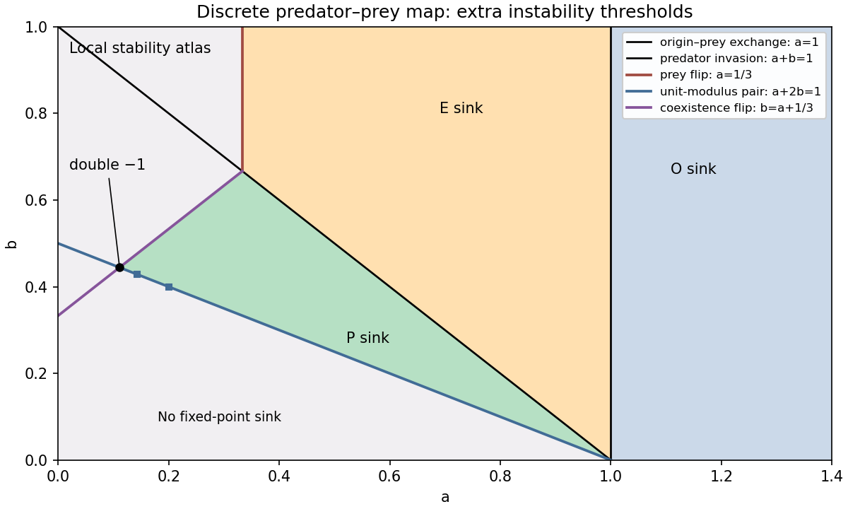


On the coexistence fixed point hasFor these give a nonreal conjugate pair on the unit circle. Nearby, while the pair remains complex, its modulus is ; increasing through one changes the modulus from greater than one to less than one. This is the candidate Neimark–Sacker bifurcation, and a nonlinear coefficient is needed to decide its direction.
Here that coefficient can be calculated explicitly. Let , , and normalize the right eigenvector and complex projection byFor deviations , the quadratic derivative isThus , and are the quadratic coefficients in . The quadratic coordinate change hasSubstitution into the map and collection of yieldsUsing and simplifies the cubic radial coefficient of a quadratic planar map toConsequently, away from strong resonances of a planar map, the bifurcation is supercritical: on coexistence is attracting, whereas on a small attracting invariant closed curve surrounds the unstable coexistence fixed point. If , its leading radius is , and its radial multiplier is . Motion on the curve can be quasiperiodic or frequency-locked into periodic motion; stability of the curve alone does not imply an irrational rotation.
Two interior values need qualification: is a 1:3 resonance, and is a 1:4 resonance. At the former is singular and the quadratic term must be retained. At the latter a cubic term remains. The resonant terms can be displayed explicitly in the same normalization. At , . The third iterate, near the resonance and after removing nonresonant quadratics, hasHere is the angular detuning. Its nonzero stationary solutions have and three phases; they constitute a saddle three-cycle. Indeed the two leading real exponents at these solutions are , of opposite signs. Therefore no ordinary attracting-circle conclusion follows arbitrarily close to the exact 1:3 point.
At , the cubic resonant normal form isThe extra coefficient follows from and . Its radial cubic damping is uniform since . The slow angular equation is , so fourfold phase locking must be considered. For example, varying at fixed gives . The locked branches satisfy and . For they form one attracting and one saddle four-cycle; the two branches alternate in phase. This is a resonant alternative to quasiperiodic motion on an invariant curve. The endpoints also fail the simple-complex-pair assumptions. This distinguishes the generic nearby dynamics from unjustified claims about every point on the printed interval.
Take the leading real field to be . A spatial translation gives ; a time translation gives ; spatial reflection exchanges and .
For a monomial in the first amplitude equation, covariance requires and . Hence , . At linear order only is allowed, no quadratic monomial satisfies these conditions, and the cubic possibilities are and . Reflection fixes the coefficients in the second equation. Removing the small common linear frequency correction by a rotating frame makes real. This derives the two cubic amplitude equations, rather than merely postulating them.
Let , . Taking real parts givesA travelling wave has , or its reflection, whenever . Its phase evolves at , shifting the physical oscillation frequency. The nonzero-amplitude radial eigenvalue is , while the absent mode has real growth rate . Therefore, on the supercritical side,The phase direction is neutral because of the symmetry, so stability means orbital stability. A branch with is radially unstable, whatever the transverse coefficient.
A standing wave has . Its two phases evolve together at ; the relative phase fixes the spatial position of the standing pattern. In the two intensity directions the eigenvalues are and . ThusAgain the symmetry phases are neutral and the conclusion is orbital stability. Equality leaves a continuum of mixed intensities at cubic order; equality removes cubic standing-wave saturation. These degeneracies require higher-order terms and cannot be classified by the cubic truncation. The zero state is linearly stable for and unstable for .
Forcing at preserves translation by one forcing period, which acts on the critical amplitudes as . It destroys the continuous common phase symmetry. Under the remaining spatial translation, transforms as , just like , and transforms just like . Both change sign under the remaining temporal sign reversal. They are therefore allowed linear terms in the respective amplitude equations. Spatial reflection requires their coefficients to coincide.
The resonant physical-frequency calculation gives the same result: multiplying the forcing factor by the conjugate left-going mode produces , resonant with the mode. The other term follows by reflection. Thus the leading parametrically forced counterpropagating waves obeywith the reflected equation for . The forcing phase can be absorbed into a common amplitude phase so that is real; its magnitude measures the resonant forcing strength. Higher-order forcing corrections are beyond this leading weak-forcing truncation.
Write , and . The polar amplitude equations arewith their reflected counterparts. On the equal-amplitude standing wave branch , equilibrium point requiresSquaring and adding eliminates the phase:For the candidate squared amplitudes areFor each positive root, set and . The quadratic identity ensures these define a phase. Conversely these phase equations imply the quadratic, so a nonzero phase-locked branch exists exactly when the discriminant is nonnegative and at least one root is positive.
Since , the discriminant condition is the printed for . It is sufficient under the usual above-onset supercritical assumptions , because then the plus root is positive. Without these assumptions the condition is not sufficient: satisfies it but gives . This is the positivity condition for a phase-locked standing wave, not a removable algebraic detail. The zero solution always exists and is distinct from the nonzero branch. For , the undivided equations must be used; a nonzero equilibrium point in this fixed rotating frame requires and . If , nonzero equilibrium points require and a compatible phase, with no cubic amplitude selection.
Strong enough forcing can overcome the nonlinear frequency shift, lock the sum phase to the external signal and produce a standing wave at half the forcing frequency. The difference phase remains free through spatial translation. The amplitude inequality is an existence condition, not a stability theorem: attraction requires the linearized forced amplitude equations, and nonlinear coefficients have not been restricted enough here to promise stability of every root.
For put . The equilibrium points are and , withThe positive branch is always a saddle. The negative branch is a sink for and a source for ; it is a node or focus according as is positive or negative. At the two branches meet in a saddle-node bifurcation when ; at the double zero eigenvalue with a nontrivial Jordan block gives a Bogdanov–Takens bifurcation. There are no real equilibrium points for .
The Hopf bifurcation curve is , equivalently on its positive- branch. Its frequency is . To determine the direction, shift , at this threshold; thenSet , to obtain , . A quadratic near-identity transformation, or harmonic averaging with its quadratic correction retained, gives the radial cubic coefficientwhere . The radial equation is . Hence the Hopf bifurcation is subcritical, with an unstable small periodic orbit on the stable-focus side .
The saddle's outgoing separatrix can return to its incoming separatrix, creating a homoclinic orbit. This global bifurcation cannot be detected from the equilibrium point's Jacobian matrix alone. The weakly Hamiltonian scaling below locates its curve and shows how the unstable Hopf cycle grows into the saddle loop. The final diagram includes the local saddle-node and Hopf curves and this global curve; it describes the neighborhood of the double-zero point.
Set and use the stated weighted spatial and parameter scales. Dividing the two equations by and respectively giveswhere prime now means differentiation with respect to . The Hamiltonian function satisfiesThus is conserved for .
For , let . The conservative system has a center at with and a saddle at withClosed contours in the left potential well have . At the left-hand separatrix is a homoclinic orbit, sinceIt leaves and returns to , with its left turning point at . The right separatrix branches are unbounded. The energy levels above the saddle value are open, as are the separate right-hand components of lower energy levels. For there is no nondegenerate potential well and no such saddle loop.
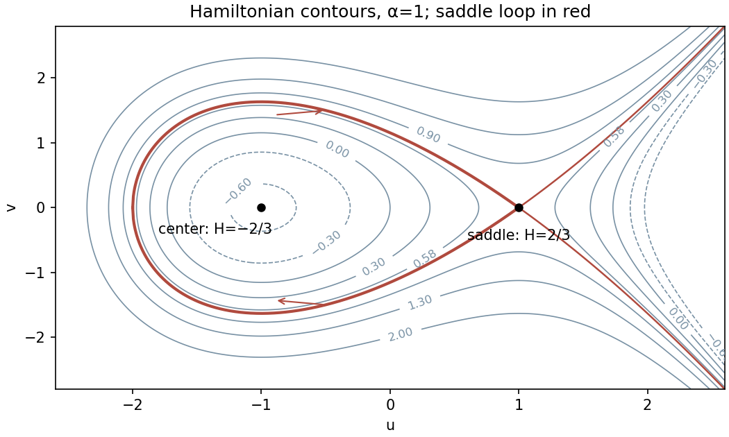
Conserved-energy contours, center and saddle loop of the leading Hamiltonian system
. Details. 
The displayed orbit has the normalization . To verify it put and . Then , , soAlso , and , exactly the same expression as . Therefore the conservative equations hold. As , ; at the orbit reaches . Its conserved energy is , so this is the required homoclinic orbit.
For a general positive set . Rescaling the verified solution givesDirect differentiation gives and , and the endpoints are . This restores the parameter dependence implicit in the normalized printed orbit.
A persistent saddle loop must return with the same energy. The Melnikov energy-balance method therefore requires, at first order,For the normalized orbit of part (c), put . Since , and ,For the general orbit has and . The energy mismatch is therefore proportional to , whose derivative with respect to is nonzero. This simple zero selects the saddle-loop curve:The remainder can be sharpened. Reversal of and interchanges and without changing the saddle-loop condition. Smoothness of the homoclinic splitting thus makes the selected an even function of , givingThe leading coefficient alone is enough to separate it from the Hopf curve . The integral hint in the PDF equals for nonnegative even integers ; for odd its integrand is odd and the integral is zero. Only even powers enter the calculation above.
Near the double-zero point, and with the stipulated absence of further bifurcations, the distinct open regions are:
- : no equilibrium points or local periodic orbits; wherever , and the flow passes through the bottleneck region.
- , : a saddle and a stable node or focus, with no local periodic orbit.
- , : a saddle, a stable focus and an unstable periodic orbit surrounding the focus. This cycle is its local basin boundary.
- , : a saddle and an unstable node or focus, with no small periodic orbit.
On the homoclinic curve the cycle becomes a saddle loop; its positive saddle trace makes the loop repelling on the cycle side. At the Hopf curve the unstable cycle shrinks into the negative equilibrium point. The node–focus discriminant curves merely change the spiral appearance and are not additional bifurcations. The impossibility of a periodic orbit for can also be seen without a picture: at a local minimum of periodic one would have and , but at its maximum the same strictly positive expression would be required to be nonpositive.
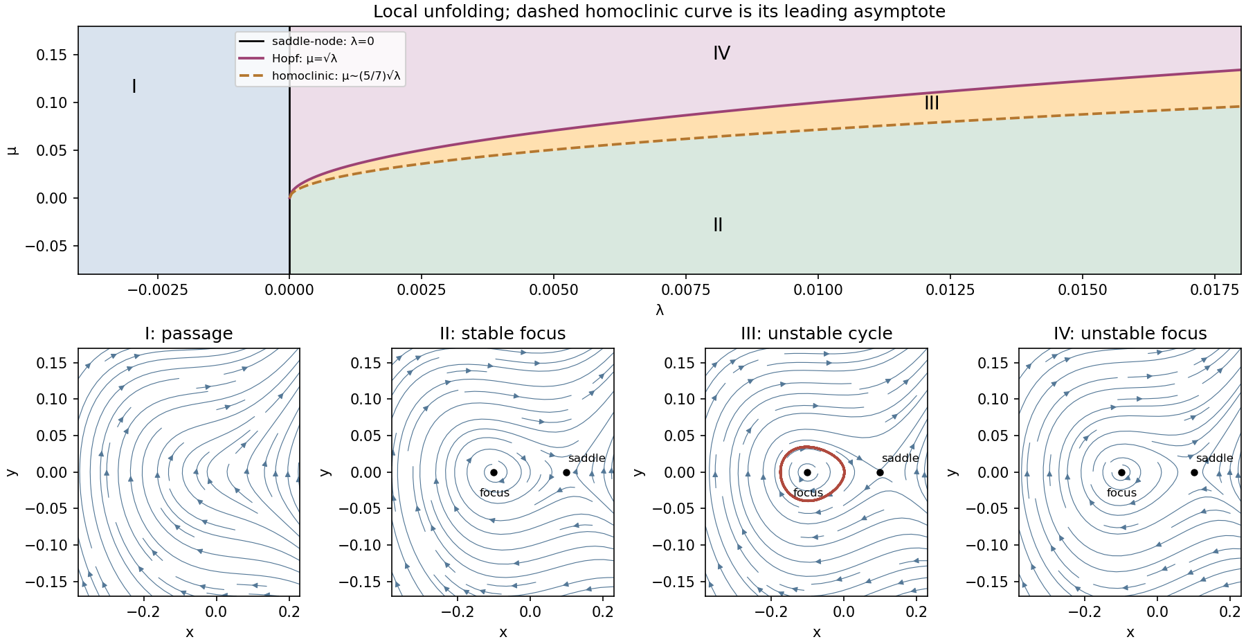
Local saddle-node, subcritical Hopf and homoclinic curves with the four nearby phase portraits
. Details. 
Articles by others on the same topic
There are currently no matching articles.