Let , and . Convolving the source terms in the Lighthill acoustic analogy with the retarded acoustic Green function, and moving their spatial derivatives outside the integral, givesThe integrals have compact spatial support. For an acoustically compact source, its size satisfies , so the source-dependent retardation is negligible at leading order. Also take . Define and . In the radiation terms the spatial derivatives act on , with . Derivatives of produce smaller near-field terms. Thus the far-field acoustic force and stress moments giveUsing gives the equivalent powers of requested. The force term is an acoustic dipole; the Lighthill stress tensor produces an acoustic quadrupole.
For a small body in low-speed flow, put . A typical unsteady force has size and time scale , whereas . ThereforeThese are the acoustic dipole Mach-number scaling and compact acoustic quadrupole Mach-number scaling. Since and outgoing acoustic intensity is of order , their sound powers scale asThus an unsteady force on the body can produce the dominant low-Mach number sound. If the integrated force or its time derivative vanishes, that dipole contribution is absent. Force on the body and force on the fluid have opposite signs.
Let the observer have cylindrical coordinates and total distance . At retarded emission time , the source-observer distance isThe retarded time relation consequently becomesSet . ThenThe observer-direction Mach number at emission is . For a constant strength and , the single retarded root has . Substituting into the moving-source field gives the rotating acoustic point source resultIn particular, on the rotation axis and the result is .
For a genuinely varying source strength, replace by in the last formula. If , the retarded relation need not be one-to-one: each retarded root contributes with in the denominator. The general result is a sum of . Dropping the absolute value and the root sum requires the subsonic assumption. At the ideal point-source expression has a caustic; finite source size and bandwidth regularize that idealization.
Use polar coordinates with ; the two faces of the screen are . Take , so the incident wave approaches from the upper half-plane, and retain the specified time dependence . Outgoing cylindrical waves then have radial factor . Define the normalized Fresnel integralThe exact Neumann Sommerfeld half-plane diffraction solution for the total spatial field isOne way to verify the Helmholtz equation is to use parabolic coordinates , . Each term has the form . The operator is , and makes its Helmholtz residual zero. At , the two Fresnel arguments coincide, while the derivatives of both the arguments and plane-wave phases cancel in pairs. Hence , which is the required normal boundary condition.
Away from the Fresnel transition regions, integration by parts gives the Fresnel tail expansionwhere is the Heaviside step function. The same expansion follows from the complementary-error-function asymptotics in NIST DLMF. Because , the tails in both terms have outgoing phase . The scattered far field is consequentlyThe first term cancels the incident geometrical optics field in its shadow, the second is its reflected plane wave and the last is the diffracted edge wave. The expansion is nonuniform at and ; the exact Fresnel expression resolves those regions. Incidence from below follows by reflecting and .
Let and . Green's second identity givesThe common Robin boundary condition makes the surface integrand vanish. Where , substitute ; a Dirichlet portion also contributes zero. The delta sources therefore give the Helmholtz Green-function reciprocityThis is a bilinear identity, with no complex conjugation. Assume the boundary-value problem has a unique Green kernel; in an exterior problem use the same outgoing radiation condition for both kernels.
For the weighted operator, assume smooth positive and set . ThenIts unweighted transpose, obtained by integration by parts, isThe associated boundary identity isTo cancel it when satisfies the given Robin condition, the required adjoint kernel satisfiesUsing these two delta sources in the boundary identity proves , the adjoint reciprocity for a weighted Helmholtz operator. As a check, , soThis is equivalent to weighted acoustic Green-function reciprocity, . Unit delta normalization is essential here. A Hermitian adjoint would instead conjugate coefficients and change the radiation convention; the requested equality uses the transpose.
Write and , with . Direct differentiation givesThus the Cole-Hopf transformation with this negative-flux convention maps the heat equation to the stated viscous Burgers equation. Conversely its residual is independent of and can be removed by multiplying by a function of .
Convolving each initial exponential with the Gaussian heat kernel givesThe resulting finite-exponential Cole-Hopf solution isIt is a softmax function average of the constant states, so and .
For , put and . Equality of the two exponents occurs atThereforeThis is an increasing viscous shock from to , moving at speed and with transition width of order . That speed agrees with the Rankine-Hugoniot condition for flux ; its concavity makes the increasing jump the entropy shock.
For general , use the shock frame . The leading coefficient in is . The endpoint coefficients coincide, and every interior coefficient is smaller by . The extremal-state asymptotics of exponential Burgers solutions therefore reduce the large- profile to the same tanh shock with states and centreAt a fixed , rather than in the moving frame, the endpoint of largest dominates. If , both endpoint rates coincide and the limiting shock is stationary. Intermediate plateaus disappear in the moving-frame limit.
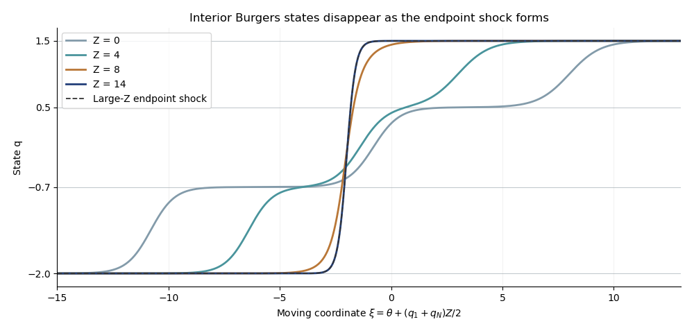
Intermediate states disappear from the finite-exponential Burgers solution in the moving shock frame
. Details. Use time dependence and consider fields independent of , with . The source-free Maxwell's equations are and . The first givesSubstitute these into the component of the second equation. The TE wave equation in a stratified magnetodielectric isBecause its coefficients depend only on , obeys the same equation. Since it is proportional to , substitution and division by giveFor a conserved transverse wavenumber , replace by to obtain the corresponding ordinary Helmholtz equations.
If “propagating along the axis” is read as strict normal incidence with no dependence, then identically. The nonzero magnetic component is , and its equation isThe equation above applies to the oblique transverse electric polarization used in the next part and also includes the zero normal-incidence solution. This distinguishes the named component from the usual transverse magnetic field.
With constant permeability, the electric equation reduces to . Insert the oblique-wave dependence and set . The inverse-square refractive-index profile givesSubstituting gives the Bessel equation of order . On either side of the profile singularity, when ,Equivalently use Hankel functions for an incoming/outgoing wave basis. If , write and replace by modified Bessel functions with argument . For , the solutions are and , with a logarithmic second solution in the repeated-root case . The constants on each side require incident-wave and boundary or matching data; the supplied singular profile alone does not choose them.
Write , . In the weak-contrast approximation , neglecting relative to gives the parabolic wave equationFor the mutual coherence , differentiating gives the exact moment equation within this wave approximation,This is an evolution equation but not a closed one. Even a jointly Gaussian random field does not make independent of , which depends on its history. Transverse statistical homogeneity alone therefore does not close the second moment. A covariance or longitudinal Markov approximation is additional information.
Under the white-in- assumption introduced in the next part, interpret , a longitudinal Brownian field with transverse covariance , and use the Stratonovich integral as the smooth-medium limit. Conversion to the Itô integral yieldsThe product rule with quadratic variation gives the closed mutual coherence in a white-noise parabolic medium equation,The two attenuation drifts contribute and the cross variation contributes . The coefficient is the white-noise covariance intensity; it replaces, rather than literally retains, the original finite pointwise variance of .
For a general colored medium and unit plane-wave input , let be the propagator of . Then the solution isA time-ordered operator exponential defines . Its expectation depends on the full longitudinal covariance; the initial Gaussian and transverse-stationarity assumptions do not specify a universal closed expression.
With the stated longitudinal Gaussian white noise and transverse statistical homogeneity, the moment depends only on . Hence . The closed equation in the previous part and initial value giveIn particular : the ensemble mean intensity remains constant for plane-wave input, even though coherent attenuation in a white-noise random medium reduces the mean complex field.
Use a consistent transverse power spectrum convention,For an isotropic spectrum, angular integration gives the isotropic transverse covariance spectrum, . ThereforeThe supplied two-dimensional Fourier transform definition has angular factor , whereas the displayed radial transform pair omits it. The latter is a normalized Hankel transform pair. If its radial spectrum is denoted , use in the integral and omit the prefactor . These are equivalent conventions; mixing them changes the attenuation rate.
Set . Substitution into the Helmholtz equation gives the first Rytov approximation equationFor the forward parabolic approximation, omit . With zero perturbation at , the Fresnel propagator then givesA jointly Gaussian random field makes a centered complex Gaussian variable. The complex Gaussian exponential moment therefore gives the first-Rytov coherent meanThe second moment here has no complex conjugation. It cannot be replaced by the positive intensity variance .
For example, let be the transverse spectrum of the covariance between depths and . The Fourier multiplier of the Fresnel propagator is , soThis supplies the requested mean in terms of medium statistics. For the longitudinal white-noise model, , which reduces the double longitudinal integral to one.
The exponential is the mean of the first-order logarithmic model. It is not a complete second-order perturbation expansion of the true mean: the omitted logarithmic term can itself have a nonzero mean. Strictly at first order, . As an independent check, the closed white-noise parabolic model gives exactlyfor plane-wave input. A truncated first-Rytov covariance expression with transverse diffraction need not equal this exact mean; omitted logarithmic terms account for the difference.
Write for the background wavenumber and . The Helmholtz equation givesThe Born approximation for scalar wave scattering replaces in this source term by . For the question's contrast , also linearize . Since , the outgoing scattered field isWithout the small-contrast linearization, replace by in this formula.
Apply the Weyl plane-wave representation. For an observation plane wholly above or below , put or , respectively, and choose with nonnegative imaginary part. Define . Substitution givesFor the lower observation plane the vertical phase has the opposite sign. This follows from the absolute separation in the Weyl identity; its version with alone applies only above the sources.
Let , and use the same two-dimensional Fourier transform for at a fixed depth. For propagating modes, and . Fourier transforming the angular spectrum in the previous part givesThe factor cancels against the change of transverse spectral variables . Hence the recoverable samples satisfyEquivalently, in terms of the requested two-dimensional transform of ,This is the Fourier diffraction theorem. It recovers Fourier samples on the two hemispheres of a shifted Ewald sphere, since the outgoing wavevector has length and the Fourier transfer is .
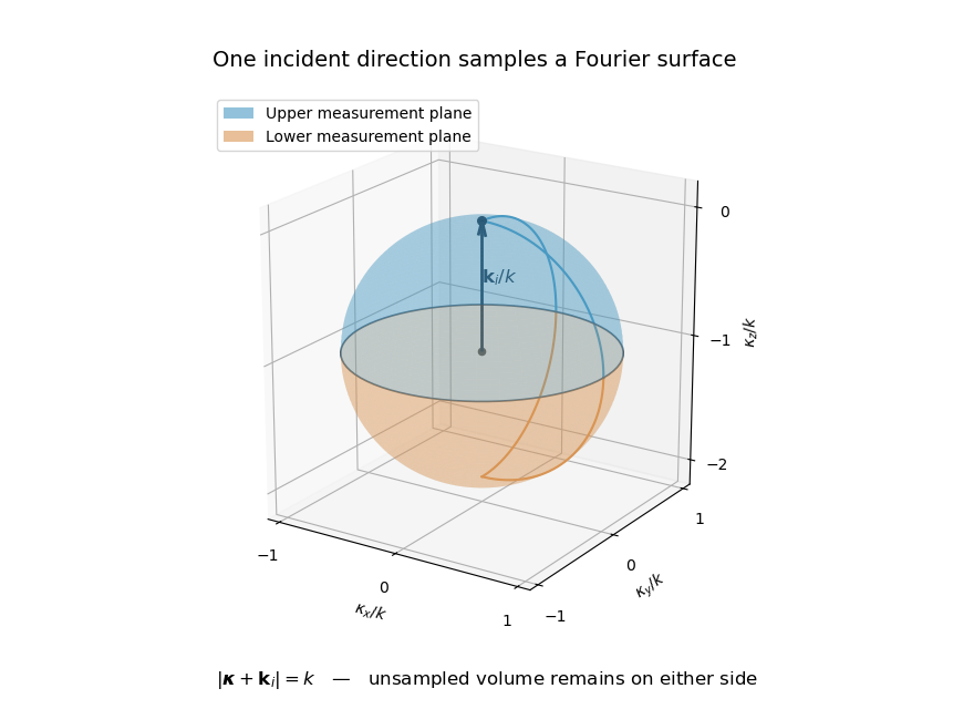


For a general three-dimensional , this is not enough to recover at every depth or reconstruct uniquely. At a fixed transverse frequency, the two planes supply only two longitudinal Fourier samples. Additional incident directions, frequencies or prior constraints are required. Thus the inverse problem as worded yields the boxed sampling relation, rather than a unique unconstrained volumetric solution.
An explicit nullspace makes this obstruction stronger than a dimension count. For any real smooth with compact support in , take the Born non-scattering contrasts at one incident directionIts Fourier transform is . On the sampled sphere, , so this polynomial factor vanishes. Nonzero real compactly supported contrasts can therefore give identical propagating data to zero contrast in this linear approximation. Their amplitude can be made small enough to keep and remain in the weak-scattering regime. In fact the associated Born field is . Applying gives the source , while compact support makes this field zero on both exterior measurement planes. Thus this example also defeats recovery from their evanescent components.
For , and the Weyl plane-wave representation contains evanescent waves. Their amplitudes decay exponentially with the distance from the scattering region. Excluding them removes high transverse spatial frequencies, including subwavelength information. Near-field measurements can in principle detect them, but back-propagating their decay exponentially amplifies measurement errors.
For propagating data, the Fourier transfer satisfies . One illumination still samples only the Ewald sphere, so this frequency bound does not imply access to every mode inside that ball. The lack of a volumetric spectrum is the separate nonuniqueness described in the previous part.
The Born approximation requires the incident field to remain a good approximation inside the scatterer. A useful sufficient smallness estimate for a weak, extended inclusion is small accumulated phase , alongside weak reflection and multiple scattering. Small pointwise contrast alone can fail for a thick inclusion or a resonance. The scalar Helmholtz and background-medium assumptions, and the extra linearization of , also belong to the model's validity conditions.
Numerically, a finite aperture windows the measured fields and limits angular and Fourier resolution. Discrete sampling must satisfy the Nyquist–Shannon sampling theorem for the retained transverse bandwidth; spacings avoid its simplest aliasing. Finite discrete Fourier transforms also introduce periodic continuation, truncation, interpolation and window errors. Noise, unresolved evanescent modes and near-grazing modes with limit reliable recovery. Refining the grid cannot by itself fill the missing three-dimensional Fourier data.
The nullspace in the Fourier diffraction theorem already prevents uniqueness, and the rapid decay of evanescent high-frequency information prevents stable recovery. Both make this an ill-posed inverse problem.
Let be the linear Born approximation operators mapping a real contrast supported in a known region to the measured fields on the two observation planes. For data , a suitable Tikhonov reconstruction from two-plane scattering data minimizesA Sobolev norm penalty can instead express a smoothness preference. Reality, known support and can be imposed as constraints. For the unconstrained complex Hilbert-space problem with the displayed quadratic penalty, write and . Its Tikhonov normal equation isTikhonov regularization selects a stable preferred estimate; it does not establish that the original two-plane data uniquely determine the true contrast.
Articles by others on the same topic
There are currently no matching articles.