Put and define the autoregressive polynomial and moving-average polynomial byFor a minimal, coprime ARMA representation, the usual simultaneous causality and invertibility root criteria for an ARMA model areThe autoregressive condition makes a stable one-sided filter and gives the causal second-order stationary process. The moving-average condition makes its inverse a stable one-sided filter, so the white noise can be reconstructed from present and past observations. If the two polynomials have a common factor, first use common factor cancellation in an ARMA model; necessary-and-sufficient root statements apply to the reduced noise-driven representation. Stationarity here is second-order stationarity; weak white noise alone does not assert strict stationarity of all finite-dimensional laws.
For , write , so . Expanding gives the Wold representationIn particular , for , and for . The coefficients are square-summable, so this series converges in mean square. Causality and invertibility identify the driver with the linear innovation process, justifying the Wold terminology. For , powers with exponent zero equal one and the formula reduces to the finite moving average.
To obtain the covariance equations, subtract and take covariance with . Orthogonality of the white noise and the causal expansion implyThus the innovation coefficients of an ARMA(1,q) process give the entire triangular system in one formula:At , use , since the autocovariance of a real stationary process is symmetric. The terms are consequently at zero, at , and the intervening partial sums as required.
For , put and . The equations becomeSubstitution of the second into the first, followed by the geometric recursion, yields the autocovariance of a causal ARMA(1,1) process:This includes : only lags survive, as for an MA(1) process.
The state-space model as printed supplies only uncorrelated white noise. That is insufficient for the claimed normal conditional distributions. For example, take normal, independent process noises taking values equally often, and independent Gaussian observation noises. With and no previous observations, is a two-component shifted mixture distribution, not normal for . Its characteristic function is , which has zeros, whereas a normal characteristic function has none. Similarly a non-Gaussian observation noise prevents the asserted conditional normal law for .
The intended scalar Gaussian Kalman recursion requires and independent of each other and of the previous state and observation history. Assume these Gaussian independence conditions, , , and the given normal filtering law. Conditional on the past, is a sum of independent normals, henceThe new observation noise is independent of and the past, so . Write and . The independent normal pair shows directly thatThe covariance comes from the common term. Applying the conditional multivariate normal distribution formula with as the conditioned coordinate gives the Kalman filter updateThe final expression verifies nonnegativity of the posterior variance.
For , defineThe recursions become and . If , then and, with ,The nonnegative solution is the steady-state local-level Kalman gain:For the limit is zero; for it lies strictly between zero and one. These are exact conditional-law results under the additional Gaussian assumptions, not consequences of the weaker printed noise description alone.
Let be proportional to the target probability density function, with . Define the ratio-of-uniforms method through the regionDraw uniformly with respect to area on and return . To prove its law, change variables from to . The Jacobian determinant is , and the allowed interval for is . ConsequentlyThe joint density of is therefore on that interval. Integrating out givesFor an already normalized density, and the region has area . The name refers to the two coordinates of a uniformly sampled region; drawing two unrelated uniforms on arbitrary intervals and taking their ratio would not give the target law.
The region usually has a curved boundary, so sampling uniformly inside it directly is inconvenient. Rejection sampling replaces it by an easily sampled envelope, usually a rectangle. Choose finite bounds withThen up to null boundaries. A general rectangle algorithm uses only independent uniform deviates: draw on , set , , and return if ; otherwise repeat. If a numerical generator returns , discard that draw before division. No knowledge of is required to run the method. Its acceptance rate is the ratio of the two areas:More generally the same area ratio applies to any finite-area envelope sampled uniformly. A change in the proportionality constant of scales both ratio coordinates and their areas consistently.
Finite rectangle bounds are a real condition, not a consequence of integrability alone. For instance is integrable, but is unbounded. A finite-area envelope for a ratio-of-uniforms region gives a general extension: choose a finite-area open envelope containing , decompose it up to null boundaries into countably many disjoint rectangles, and select a rectangle with probability proportional to its area using a uniform draw and cumulative probabilities. Use two more uniforms to sample within it, then apply the same acceptance test. This samples the envelope uniformly and has acceptance . Such envelopes exist for every finite-area measurable ; obtaining usable bounds or an effective rectangle decomposition is density-specific. The finite-rectangle version above is the usual practical implementation.
For , use the unnormalized normal density . Its ratio region isThe bound on is one because is maximized at zero. To bound , maximize for . Its derivative vanishes at , giving . Thus the normal ratio-of-uniforms envelope is , .
Draw independent , set and , and accept precisely whenreturning . Equivalently compare logarithms to avoid underflow. Since , the region area is and the rectangle area is . ThereforeIt is independent of the normal scale. In the diagram the vertical coordinate is normalized by , so the same shape works for every positive scale.
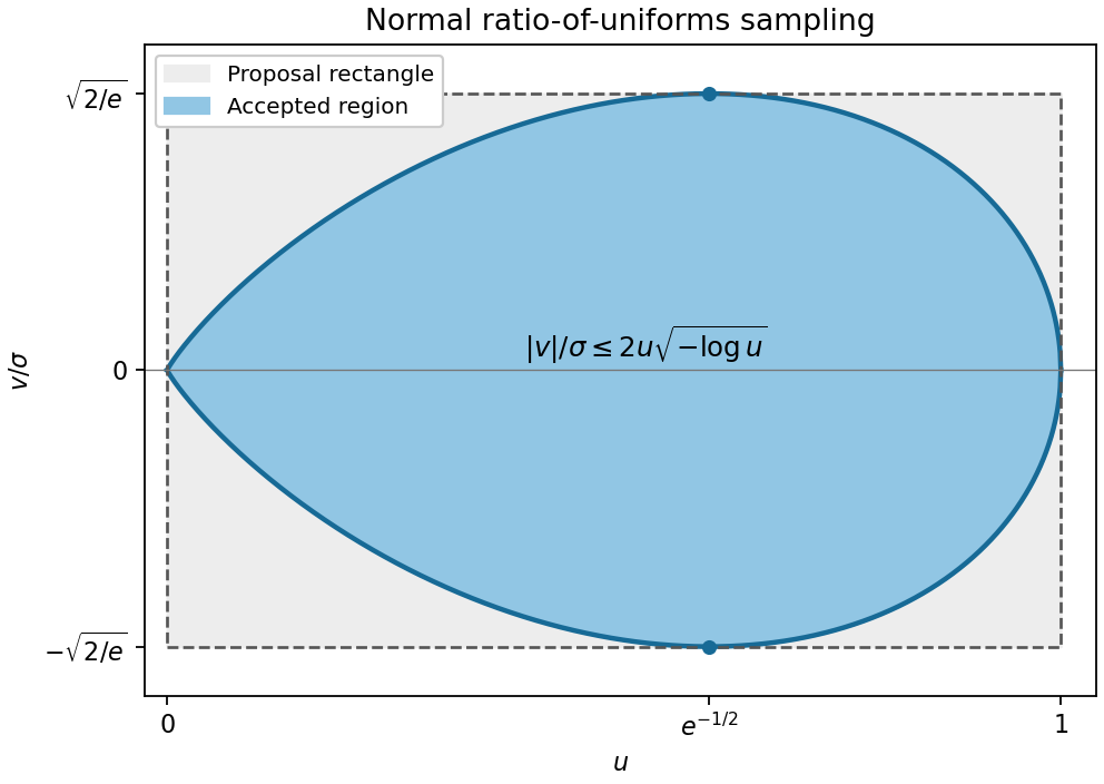
Normal ratio-of-uniforms region and its minimum axis-aligned rejection rectangle
. Details. 
For independent standard Cauchy distribution draws , the code averages the indicators . Each is a Bernoulli random variable with parameterHence it is an unbiased estimator of that tail probability, and independence givesThe variance is finite even though the underlying Cauchy draws have no finite mean: the variables being averaged are bounded indicators, not the Cauchy values themselves.
For with uniform on ,Thus has a Pareto distribution and is the importance sampling proposal, concentrated on the required tail. The target tail integrand is , so its importance weight isThe function returns . Since , it is an unbiased estimator. For its second moment,An antiderivative is , so the integral is . Independence of the proposals givesThis is importance sampling of a Cauchy tail, with weights between and . Their narrow range explains the much smaller variance than the indicator estimate, without appealing to nonexistent Cauchy moments.
There is a genuine normalization error in the printed function. Write independently, and . The internal sum produces a scalar; taking its mean does not divide by . The literal returned value is thereforeSince and , its expectation isIt does not estimate unbiasedly unless , and no fixed control variate coefficient removes this bias. In particular the actual call with returnsThis is an instance of summing before taking a mean changes Monte Carlo normalization.
The intended corrected method replaces the sum by a sample mean:It uses symmetry to write the tail as , then Monte Carlo integration on a bounded interval, and finally a mean-zero control variate. For the intended estimator is , whose summands are smooth and bounded. Keeping the average normalization, andDifferentiating this quadratic gives the Cauchy tail control variate on a bounded interval coefficientHere , , so . AlsoConsequentlyThe negative sign is consistent with decreasing and increasing. One may estimate the covariance and variance using a separate pilot sample and fix the resulting coefficient for a fresh sample. This coefficient minimizes the literal function's variance as well, but its missing factor of still leaves the bias above.
For a target probability density function and a proposal distribution with density , the Metropolis–Hastings algorithm starts in the target support and repeats: propose , draw an independent uniform , and move to ifOtherwise retain . A zero reverse-proposal density makes the acceptance zero. Unknown multiplicative constants of cancel. For distinct states,which is symmetric in the states. Together with the probability of holding at the current state, this proves detailed balance and invariance of . Successive values form a dependent Markov chain; convergence from arbitrary initial states additionally needs the appropriate irreducibility and aperiodicity, not just this invariant-density identity.
The Gibbs sampler updates a coordinate using its full conditional distribution while keeping the others fixed. For coordinate , write and . Its proposal replaces by . The MH ratio, interpreted on this one-coordinate proposal space, isThus every Gibbs coordinate update is an MH update with acceptance one. A random choice of coordinate gives a mixture of these invariant kernels; a deterministic sweep gives their composition. Both preserve . The latter composition need not be reversible, so the special-case statement is about the coordinate kernels, not a claim that every entire systematic sweep is one reversible MH kernel.
At , complete the square:For fixed , all factors not involving enter its conditional normalizing constant. Interchanging the roles of the coordinates givesThese are the full conditional distributions of the standard bivariate normal distribution with correlation .
A systematic Gibbs sampler starts at a chosen and, at each sweep, draws independent standard normals and setsThe second update uses the newly drawn . Both coordinate updates preserve the target by part (a), hence so does the sweep. The Gaussian two-coordinate Gibbs recursion is explicitlyan AR(1) recursion with innovation variance . Its stationary variance is one, and its correlation at sweep lag is , displaying the dependence of the sample.
The printed general- expression has a separate normalization defect: for its integral is , not one, since the exponent has covariance , whose normalizing denominator is . Retaining that exponent requires in the prefactor. The requested target is already normalized, so this defect does not alter the conditional distributions above.
Use the random-walk proposal specified by its centre and covariance: for the current state draw independently standard normal and setIts properly normalized density of the proposal distribution isIt is symmetric: . This is a centred-at-the-current-state proposal, rather than an unshifted draw from the density notation in the source. The random-walk Metropolis algorithm consequently needs only the target ratio. Put . ThenAn independent uniform decides the move; on rejection both coordinates remain at their previous values. A proposal with lower is always accepted. This construction uses the joint density directly, without needing either conditional distribution. Its continuous positive proposal density supplies communication over the target support, and the holding probability avoids a deterministic periodic transition pattern.
Tune the proposal scale using pilot runs on a grid of candidate values. After allowing for initial transients, compare the effective sample size of a Markov chain per unit computation time for representative functions, such as both coordinates and a quadratic function. Equivalently inspect their integrated autocorrelation time, using . Choose a useful scale and keep it fixed for the production run. Another pilot criterion is the average squared accepted displacement, possibly in coordinates standardized by the target covariance, which balances move size and rejection.
Acceptance alone is not an efficiency criterion. As , proposals are almost the current state, so acceptance tends to one while exploration becomes arbitrarily slow. Very large scales propose mostly low-density states and produce long sequences of identical values. The proposal scale and random-walk Metropolis efficiency trade-off requires both movement and acceptance; neither maximizing nor merely reporting the acceptance probability guarantees a useful sample. With strong correlation, an isotropic proposal also struggles with the target's narrow direction; covariance-scaled proposals can improve this geometry beyond tuning one scalar variance.
The observed-data likelihood function integrates out the latent variable:Choose an initial parameter with positive likelihood. At iteration , the E-step of the EM algorithm forms the entire expected complete-data log-likelihoodThe expectation is under the conditional missing-data law at the old parameter, while the argument remains free. The M-step then choosesThe observed data stay fixed throughout. This is not obtained merely by substituting the conditional mean of into a nonlinear log-likelihood: the expectation of all required complete-data terms must be taken. A generalized EM step only requires , which suffices for the monotonicity proved next. Exact maximization assumes that an admissible maximizer exists.
Write and . Assume the likelihoods are positive and the expected log likelihoods used in the step are finite. On the support where , let . Integrating over that support givesIt is an equality when the candidate joint density has no additional mass outside the old support. Concavity of the logarithm and the Jensen inequality now implyThus the argument does not silently require an identical support at every parameter. The M-step selects a value whose right-hand side is nonnegative, proving EM likelihood monotonicity:When the conditional densities allow finite divergence, the same calculation has the informative exact formThe Kullback-Leibler divergence is nonnegative, since . This also explains why an increase of the surrogate objective guarantees an increase of the observed objective, while equality of the two likelihoods is possible.
EM likelihood monotonicity makes EM an ascent method, not a global-optimization theorem. If the log-likelihood is bounded above along the iterates, its nondecreasing values converge. That alone does not show that the parameters converge, nor that any limiting parameter is a global maximum-likelihood estimator. Under additional regularity, accumulation points can be stationary; local maxima, other stationary points or flat sets can depend on initialization. Multiple starting values and comparison of the achieved observed likelihoods are therefore useful.
The upper-bound hypothesis is substantive. In a finite mixture model with a freely shrinking normal-component variance, placing one component at an observed value can make the likelihood unbounded while other components cover the remaining observations. In that situation monotonicity provides no finite maximum to converge to. EM may also improve very slowly, and a small change in likelihood alone is not proof of an accurate global solution. The guarantee in part (b) is nondecrease, not strict increase at every iteration.
Both EM algorithm and data augmentation exploit a latent completion , but they use it differently. EM takes a conditional expectation of the complete-data log-likelihood and then maximizes over the parameter, producing a deterministic sequence of point estimates when the M-step is uniquely specified.
In Bayesian data augmentation, choose a prior distribution and targetAlternate the Gibbs sampler updatesThese are stochastic draws from full conditional distributions, not an expectation followed by maximization. Their invariant law is the augmented joint posterior, and discarding gives posterior inference for , including uncertainty rather than only an MLE. A sampled completion followed by maximization would instead be a stochastic EM variant. Individual likelihood values along a data-augmentation chain need not increase: the chain is designed to sample a posterior, not to ascend the likelihood.
Articles by others on the same topic
There are currently no matching articles.