For an autonomous ordinary differential equation, the chain rule gives . The formula is therefore a multiderivative multistep method. Insert the exact solution and expand the two earlier values about :The unscaled local truncation error isThe coefficients through vanish, but the fourth-order coefficient does not. Hence the method has order three, not four: the one-step residual is for an order- multistep formula. Its zero-stability polynomial is , with a simple unit root and the other root inside the unit disk. Thus the stated order is also the convergence order for smooth solutions, starting errors , and the nearby implicit solution branch, by convergence of a zero-stable multiderivative method.
Yes: this is an A-stable third-order method. Its second derivative is essential; the Second Dahlquist barrier applies to ordinary first-derivative linear multistep methods, not this multiderivative multistep method.
Apply the Dahlquist test equation and put . The amplification polynomial isWe verify the root condition for a multistep method throughout . For a quadratic with , the complex quadratic Schur criterion isfor both roots to be strictly inside the unit disk. Here is a brief justification of the criterion rather than just a root plot. Set . The polynomial is , where and . Its two roots are inside precisely when . On the unit circle , and , so the Rouche theorem equates its interior root count with that of . A boundary zero of would also be a boundary zero of the transformed polynomial, which the strict inequality excludes. This proves the strict criterion; the non-strict form follows by continuity, with any unit root simple because .
For the present polynomial it is enough to show , except at . Write , , and put , . ThenDirect expansion gives the nonnegative factorizationEvery term is nonnegative, and the sum is strictly positive unless . Also , so the criterion applies. For every nonzero in the closed left half-plane both amplification roots are strictly inside the unit disk. At they are and , and the unit root is simple. ThereforeThis proof establishes stability of both the principal and parasitic modes, including on the imaginary axis.
In the variational convention needed here, a positive definite symmetric operator on a real Hilbert space satisfiesFor a bounded operator on the whole space, symmetry is self-adjointness. On a complex Hilbert space, the corresponding convention is Hermitian positivity; the quadratic expression is real. Strict positivity should be distinguished from uniformly positive definite symmetric operator coercivity, which requires a fixed such that .
Symmetry matters in a real space. If “positive definite” means only the inequality for the quadratic form, the next variational assertion is false: has , but its skew part disappears from that form. Its Euler-Lagrange equation is , not . Thus the usual symmetric/Hermitian convention, or an explicit symmetry assumption, is required.
For a real Hilbert space, differentiate along an arbitrary direction :The last equality uses the symmetry in the definition of a positive definite symmetric operator. Vanishing of this first variation for every is equivalent to , givingIf solves it, expand the functional about to findThis is strictly positive for nonzero , so is the unique minimizer. Conversely a minimizer has zero first variation and solves the equation. On a complex Hilbert space, use the real functional and real directional derivatives; varying and yields the same result.
This proves the quadratic variational principle for a symmetric positive operator, conditional on existence. Strict positivity in infinite dimension does not by itself guarantee a minimizer for every : on , the operator is strictly positive, but would require the non-square-summable solution . A coercive bilinear form supplies existence through the Lax-Milgram theorem under its usual boundedness assumptions.
Interpret the differential expression as , with a suitable differential-operator domain and the stated clamped boundary conditions. For sufficiently smooth in that domain, twice integrating by parts givesThe boundary term vanishes because at both ends. For real coefficients this form is symmetric/Hermitian. In particularIndeed nonnegativity follows from and . If the integral were zero, almost everywhere in the interval, so would be affine. Its endpoint values then force . This proves strict positivity on the intended clamped domain and gives the weak formulation of a clamped fourth-order equation.
There is a genuine domain issue in the literal wording. The closure of clamped smooth functions in the stated L2 norm is all of , since it contains the dense set . Boundary traces are not retained by that closure, and a fourth-order expression does not define an operator on every element of . For example , satisfy the given sign conditions, but belongs to this closure and makes a distribution rather than an function. Even a general twice-smooth function need not have the four derivatives required by the classical expression.
A rigorous classical repair is to take smooth enough coefficients, for example , , and use a clamped domain such as in , with the appropriate operator realization. A weak repair uses the clamped second-order Sobolev space and the form just displayed, with hypotheses ensuring its boundedness and closure; uniform positivity makes it coercive there. The integration-by-parts and strict-positivity proof does not need that stronger uniform bound, but existence and completion statements must not be inferred from the original closure alone. The printed with an expression in is also a harmless variable-name mismatch; the calculation consistently uses .
Put . The spatial operator is the sum of a centred difference and a dissipative second-order forward advection stencil in . For a smooth function, their Taylor expansions giveThus the leading spatial local truncation error is , generally nonzero. The semidiscretization is second order in space. Time has not yet been discretized, so there is no separate time order or time-step condition at this stage.
Use von Neumann stability analysis on the infinite grid. For the Fourier mode , the semidiscrete eigenvalue isIts real part is nonpositive for every frequency. The mode evolves by , whose modulus does not grow. The discrete Fourier transform and Parseval identity therefore yieldwith a bound independent of , where . Hence the semidiscrete method is stable. Frequencies with are nondissipative rather than unstable.
The same sign can be seen directly by summation by parts: the centred operator is skew-adjoint, and for the unitary shift ,This is an energy version of the dissipative second-order forward advection stencil. A subsequent time integrator would need its own stability condition; semidiscrete stability does not assert that every fully discrete method is stable.
For and step , a collocation Runge-Kutta method constructs a polynomial of degree at most on satisfyingThe step value is . Thus the differential equation holds exactly at the prescribed collocation nodes, while the initial value fixes the integration constant. For a smooth vector field and small enough , the implicit stage equations have the local solution branch continuing the zero-step initial state; arbitrary large steps need not have a unique nonlinear solution.
Let be the Lagrange interpolation basis. Set and . Since is a polynomial of degree at most , the collocation conditions giveIntegrate from zero to and to one to obtainThese are the stage and update equations of a Runge-Kutta method with nodes . Conversely, stages satisfying these equations reconstruct by integrating the displayed interpolation polynomial, so the equivalence works in both directions. Because , they also satisfy the collocation tableau row-sum identity .
The collocation order theorem identifies the classical order with the order of its interpolatory quadrature. If integrates every polynomial of degree at most exactly, but fails for some polynomial of degree , then the collocation method has order for sufficiently smooth differential equations and the local implicit stage branch. With nodes, .
Equivalently, put . If its first moments vanish,and the next does not, then . Polynomial division explains the quadrature part: any polynomial through degree is a remainder of degree below plus times a polynomial of degree below . The remainder is integrated exactly by interpolation, and the remaining integral vanishes. Conversely a nonzero next moment is an explicit failed quadrature test. The differential-equation order assertion is the collocation theorem being stated here. In particular Gauss collocation methods achieve , Radau IIA methods achieve , and endpoint-including Lobatto IIIA methods achieve for .
The tableau as printed is not a collocation tableau. Its second stage row is , whose sum is , while the corresponding printed node is . This violates the collocation tableau row-sum identity. The original PDF confirms this coefficient; it is not only a TeX transcription defect.
The required integrated basis at nodes isso direct integration givesThus replacing the last stage coefficient by gives the intended two-stage Radau IIA collocation method. Its quadrature moments areIt integrates quadratics exactly but not cubics, so the collocation order theorem gives order three. Independently, , confirming the remaining third-order Butcher order condition.
For completeness the literal printed Runge-Kutta method has only order one. For the autonomous equation , the Taylor expansion of its stability function beginswhereas . Since , it is consistent, but this discrepancy already rules out order two. Therefore neither the requested equivalence nor the third-order conclusion is true without the stated coefficient repair.
Write and collect only the interior values, so the actual vector dimension is . The PDF's matrix size and its indices are inconsistent with the declared interior grid ; neither affects the following stability argument when the interior indexing is used consistently.
Use the discrete L2 norm , extending by zero to the boundary. Let be the horizontal flux operator and the vertical one. Each face coefficient is shared by its two adjacent grid values, so summation by parts givesAll boundary-face terms are included. Positivity of makes symmetric negative definite on the interior grid: zero in either energy sum forces each corresponding grid line to be constant, and its zero boundary endpoint forces that constant to vanish. ConsequentlyThis bound is independent of the spatial mesh, proving semidiscrete stability. No time integrator or time-step restriction has yet been introduced.
Put and , keeping the spatial grid fixed for the temporal error assertion. The matrix exponential expansions giveHence the Lie-Trotter splitting commutator error isThe energy estimate from part 1 makes , and contractions, so both and have norm at most one. Telescope their th powers:For , this givesThus the Lie-Trotter splitting has global temporal error . The constant here may depend on the fixed spatial operators; a mesh-uniform joint-limit error estimate needs additional regularity and commutator bounds. If and commute, this particular exponential splitting is exact, but variable diffusion coefficients generally remove that commutativity.
The Padé approximant of the exponential is . Replacing each exponential in its original order gives the split Crank-Nicolson methodwith the analogous definition for . Operationally, first solve the substep and then the substep. The matrices , are invertible for every , since are symmetric negative definite.
An orthonormal eigenbasis of diagonalizes . Its eigenvalue for isTherefore , and similarly . Submultiplicativity gives the contractivity of split Crank-Nicolson diffusion:No commutativity or simultaneous diagonalization is needed for this product bound. This proves unconditional discrete stability, not positivity of every stencil weight or unconditional maximum-norm monotonicity. Nor do the individually second-order rational substeps make the ordered splitting second order: when , its leading splitting defect remains .
A-stability removes the scalar linear decay restriction on the step size; it does not replace accuracy, nonlinear solvability or a suitable system norm. Its importance is clearest for a stiff differential equation, where rapidly decaying modes coexist with slowly varying quantities of interest. On the Dahlquist test equation , the exact solution decays for . A stable time integrator should not turn that decay into numerical growth.
For a one-step method write , where and is its stability function. Its linear stability domain consists of parameters with and a well-defined update. The method is A-stable when this domain contains the closed left half-plane. A consistent order- one-step method has near zero, but that local agreement alone says nothing about stability at large negative .
For a Runge-Kutta method with stage matrix , weights and , eliminating the stages on the test equation givesAn explicit finite-stage method has a polynomial . A nonconstant polynomial is unbounded along the negative real axis, so no consistent explicit Runge-Kutta method is A-stable. The explicit Euler method, with , is stable in the disk and on the negative real axis only for . A stiff mode with a large negative eigenvalue therefore forces an unnecessarily small step even after its exact contribution has almost disappeared.
The Backward Euler method has . For , , so it is A-stable. The trapezoidal rule hasand is also A-stable. The implicit midpoint method has the same scalar stability function, although its nonlinear update differs from the trapezoidal rule. The first method has order one and the latter two order two. Their implicit solves trade greater work per step for freedom from the scalar stiff stability restriction.
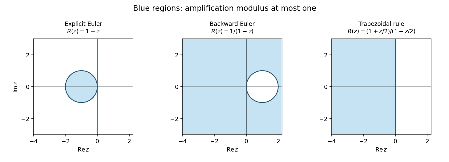
Absolute stability domains of explicit Euler, backward Euler and the trapezoidal rule; shaded regions satisfy modulus of the amplification factor at most one
. Details. 
Damping of very stiff modes separates A-stability from L-stability. For a one-step method, the latter additionally requires as tends to infinity in the left half-plane. Backward Euler method satisfies this. The trapezoidal and midpoint rules instead have along the negative real axis: a very stiff mode can alternate in sign with little damping even though its amplitude remains bounded. L-stability is often preferable for diffusion and rapid relaxation, while retaining oscillatory modes can be desirable in conservative dynamics.
For a linear multistep method, writeIts test-equation amplification roots satisfy . Absolute stability requires every root to lie in the unit disk or on its boundary with all unit-modulus roots simple; all parasitic modes matter. At this is the zero-stability root condition. Consistency requires and , and the Dahlquist equivalence theorem combines consistency and zero-stability to characterize convergence. Thus a claim of stability obtained by canceling a common factor is not a proof about the original recurrence and its arbitrary consistent starting data.
Explicit linear multistep methods cannot be A-stable either. If and , some lower coefficient of becomes unbounded as , while the leading coefficient stays fixed. If all roots remained in the unit disk, every coefficient-to-leading-coefficient ratio, an elementary symmetric function of those roots, would remain bounded. This contradiction forces an unstable root.
An important implicit example is BDF2 method, whose characteristic equation is . A unit root givesThe leading coefficient vanishes only at , outside the left half-plane. Near a small negative , both roots are inside the disk; no unit-circle crossing can occur in the connected open left half-plane. On the imaginary axis the boundary equality can occur only at , where the roots are . Hence BDF2 is A-stable and its two roots tend to zero for very large negative , giving strong stiff-mode damping. This is a complete boundary-locus argument, not just a boundary plot.
The Second Dahlquist barrier says that a convergent A-stable ordinary linear multistep method has order at most two. This theorem does not limit implicit Runge-Kutta methods or multiderivative multistep methods. In particular the A-stable third-order two-step multiderivative method in question 1 uses and satisfies different order conditions. Among collocation Runge-Kutta methods, the standard family results give Gauss collocation methods order with diagonal Padé approximants to as stability functions, and Radau IIA methods order with subdiagonal approximants. Both families are A-stable; the Gauss functions have a nonzero limit at infinity, whereas Radau IIA is L-stable. The corrected two-stage right-Radau method, for example, haswhich matches the exponential through cubic order and tends to zero at infinity. Its poles lie in the right half-plane. For , , direct subtraction givesproving its A-stability directly.
Sectorial A-alpha stability relaxes the requirement to a sector around the negative real axis, useful when the spectrum of a stiff problem remains in that sector; higher-order backward differentiation formulas illustrate the usefulness of this weaker requirement. For a normal linear system , unitary diagonalization reduces the numerical update to its scalar factors . For a nonnormal system, a scalar eigenvalue test alone does not give a uniform bound in the chosen norm. Nonlinear stability is different again: B-stability asks for contractivity when , and algebraic stability of a Runge-Kutta method is a standard sufficient criterion. Thus A-stability addresses a precise and valuable linear test, while step selection still has to meet accuracy requirements and the actual implicit equations must be solved on the relevant branch.
Eigenvalue analysis proves mesh-uniform stability when it is accompanied by control of eigenvectors or an energy norm; the signs of eigenvalues alone are insufficient. For an evolution equation, the method of lines first produces . A time integrator then gives an amplification matrix , for example for a Runge-Kutta method. The useful stability requirement on a fixed physical time interval iswhere is independent of the refining spatial and temporal meshes. The semidiscrete analogue is for . These are bounds on propagation of initial errors and residuals, not merely statements that each finite matrix has a bounded solution over its own finite time interval.
If is a normal matrix in the chosen discrete inner product, it has a unitary eigenbasis. ThenFor dissipative problems it is sufficient that every lie in the integrator's linear stability domain. A diagonalizable family also suffices if its eigenvector matrices have uniformly bounded condition numbers: the same maximum is multiplied by . Without that uniform bound the argument does not establish mesh stability. For finite-time estimates, an amplification modulus can also be acceptable; strict contraction at every step is a stronger property.
For a constant-coefficient stencil on the full lattice or a periodic grid, von Neumann stability analysis provides the eigenvectors explicitly. A Fourier mode diagonalizes each translation-invariant spatial difference, giving a scalar symbol or a small matrix symbol for a system. The discrete Fourier transform and Parseval identity turn a uniform modal bound into an actual discrete L2 norm bound. The two-dimensional stencil in question 3 has , so its continuous-time amplification is contractive; a later time integrator must still be checked. With boundaries one must analyze the boundary rows as well: a whole-line Fourier symbol cannot detect an unstable boundary closure.
For the heat equation on a unit interval with zero Dirichlet data, the centred second difference has a sine eigenbasis and eigenvaluesExplicit Euler method multiplies mode by . Requiring all factors to have modulus at most one yields on a given grid, and the sharp grid-independent sufficient limit isThese parabolic time-step restrictions express the growth of the largest-magnitude diffusion eigenvalue like . Backward Euler method instead has factor and the Crank-Nicolson method factor , both bounded by one for every . Their unconditional stability follows from A-stability, with much stronger damping of the shortest scales for backward Euler.
For , , explicit time stepping with a backward spatial difference givesThus the upwind finite difference scheme is contractive exactly for , a Courant–Friedrichs–Lewy condition matching the direction and speed of information propagation. A centred spatial difference has purely imaginary eigenvalues, and forward Euler gives . Under a fixed positive hyperbolic Courant number, high-frequency data grow by a fixed factor in each of steps, proving instability as the mesh is refined. This is not a claim that no exceptionally small coupled step can ever give a finite-time bound: if , the excess per step is only , but the usual hyperbolic scaling is unstable. Higher-order explicit integrators can possess nontrivial imaginary-axis stability intervals and are then suitable for skew-adjoint advection or the energy-form first-order wave equation.
Variable coefficients usually prevent Fourier diagonalization, but may preserve a self-adjoint spatial operator. The positive-face diffusion discretization in question 5 is an example. Its discrete energy identity makes symmetric negative definite, so a unitary eigenbasis still exists even without a closed eigenvalue formula. More generally, a dissipative operator in a discrete energy inner product obeyswhich directly proves a uniform semigroup estimate. The dissipative Cayley-transform contraction also follows without normality: for ,Taking proves contraction of the Crank–Nicolson factor. The contractivity of split Crank-Nicolson diffusion then follows from multiplying two contraction bounds; simultaneous eigenvectors of the two directional matrices are unnecessary.
The negative spectra do not imply uniform semidiscrete stability example shows what can go wrong. LetBoth eigenvalues are for every mesh, but applying the propagator to the second unit vector at gives norm at least . The evolution is therefore not mesh-uniformly stable. For a discrete matrix, a unit-modulus eigenvalue with a nontrivial Jordan block gives powers growing polynomially in the step number. Even strictly interior eigenvalues can allow large transient growth when eigenvectors are badly conditioned. A pseudospectrum or numerical range of an operator, and especially a direct energy estimate, can reveal behavior missed by eigenvalues.
A resolvent estimate provides another way to see the needed uniformity. If for every , then for ,This shows directly that a uniform power estimate imposes more than the location of the spectrum. Conversely, resolvent-to-power estimates in varying dimension must themselves be uniform; a bound with constants depending on the number of grid points is not enough.
For a linear multistep method, each spatial eigenvalue gives an amplification polynomial, and all roots must satisfy the root condition for a multistep method, including simplicity of any unit-modulus root. Merely following the root approximating misses parasitic modes. The temporal and spatial analyses must therefore be combined with the appropriate zero-stability and uniform modal bounds.
Finally stability connects to convergence. If the exact grid samples have normalized residual and the error obeys , iteration givesA residual tending uniformly to zero then gives convergence on . For a well-posed linear initial-value problem and a consistent linear finite-difference approximation, this is the forward implication of the Lax equivalence theorem. The practical conclusion is to analyze the full operator including boundaries, select a time method whose stability region contains the relevant scaled spectrum, and verify that eigenvectors or an energy estimate make the resulting bounds uniform as the grid is refined.
Articles by others on the same topic
There are currently no matching articles.