Past exam of the mathematics course of the University of Cambridge / 2012 / iii / Paper 41 (Biostatistics)

Screening applies the eligibility criteria for a clinical trial before treatment allocation. It identifies the population to which the comparison pertains and excludes individuals for whom the intervention or measurements are unsuitable. Recording potentially eligible individuals also helps describe recruitment and assess external validity. It should precede randomization so eligibility is not decided using knowledge of the allocated treatment.

Obtain informed consent so that participation in the clinical trial is voluntary and based on an understanding of its procedures, potential benefits and risks, alternatives and withdrawal arrangements. Consent before allocation prevents willingness to participate from being selected according to the known treatment assignment.

Measure baseline covariates before the intervention can change them. These measurements describe the recruited population, permit assessment of covariate balance, and provide prognostic predictors that can improve statistical efficiency. In particular, including prognostic baseline covariates in a linear regression reduces unexplained outcome variation without conditioning on a treatment consequence.

Randomization makes assignment independent of the participants' pre-existing potential outcomes, giving an unbiased comparison of allocation groups under the usual trial assumptions. It therefore protects against baseline confounding, including from unmeasured factors, and supplies an assignment distribution for inference. Allocation concealment protects this step from recruitment decisions based on the upcoming assignment. It does not guarantee exact balance in every realized sample.

Use a baseline-adjusted linear regression for an intention-to-treat analysis:Condition on the observed baseline covariates and assignment. The parameter of primary interest is $\beta$, the mean effect of assignment to the experimental intervention, under this constant-effect conditional mean model. Independent normal distributions with common variance give the usual Gaussian likelihood and regression inference. Prognostic baseline covariates improve precision by explaining outcome variability.

Do not include the actual intervention-use variable $D_i$ as an ordinary adjustment variable for this estimand: it is measured after assignment and can mediate the effect being estimated. Post-randomization adjustment changes a treatment estimand; the resulting coefficient on $Z_i$ would generally represent a different comparison. Participants remain in their assigned groups even when adherence differs.

Let $R_i=1$ indicate an observed outcome. Fitting the conditional outcome model to responders requireswith a positive observation probability over the relevant predictor support. This is conditional missing at random for the predictors used in the regression: after conditioning on them, observation must not further select participants by their unobserved outcome. It gives $f(Y_i\mid x_i,Z_i,R_i=1)=f(Y_i\mid x_i,Z_i)$, the complete-case regression under conditional missing at random condition. Correct specification of the conditional mean model is also required. Missing completely at random is sufficient but stronger; simply assuming missingness depends only on a post-randomization variable excluded from this model would not suffice.

Write ${\mu }_i=\alpha +\beta z_i+{\gamma }^{\mathsf{T}}{x}_i$ and let $f_i(y)={\sigma }^{-1}\varphi ((y-{\mu }_i)/\sigma )$ be the normal distribution density. Set $q_j(y)=\mathrm{expit}({\eta }_j+\theta y)$, where $q_j$ is the probability that attempt $j$ is unsuccessful conditional on the preceding attempts being unsuccessful. This is a sequential response selection model. For first-attempt success, the observed outcome and attempt count contributeThis likelihood conditions on baseline and assignment; the displayed response probabilities do not use $d_i$. No factor for random allocation is needed when conditioning on its realized value.

Four unsuccessful attempts have conditional probability ${\prod }_{j=1}^4{q}_j(y)$. The outcome is then unobserved, so the observed-data likelihood integrates over it:This is a probability, whereas a responder contributes a joint density in the observed outcome. The sequential response selection model keeps outcome-dependent nonresponse in the likelihood; evaluating the product at an imputed mean would not be this likelihood.

Within the displayed sequential response selection model, $\theta =0$ makes every attempt's nonresponse probability independent of $Y$, and hence gives the outcome-independence needed for complete-case analysis. The estimate $\hat{\theta }=0.38$ suggests that larger outcomes are associated with greater odds of an unsuccessful attempt. Per one-unit outcome increase, the fitted odds ratio is $e^{0.38}\approx 1.46$, with the reported interval transformed to $(e^{-0.06},e^{0.82})\approx (0.94,2.27)$.

The confidence interval for $\theta$ includes zero, so there is no rejection of outcome-independent missingness at the five-percent level within this model. This does not establish that the missing at random assumption is true: the interval also allows appreciable outcome dependence, and inference depends on the chosen selection model. The intercepts describe response levels, not independence from the outcome. Nor can the respondents' mean and standard deviation establish the missing outcomes' distribution. There are $300-211=89$ unobserved outcomes, about $29.7\%$, so conclusions about the full trial depend materially on the missingness assumptions.

The two independent binomial distributions give fitted event probabilities $24/99$ and $12/100$. Their odds ratio and log odds ratio areUsing the log odds ratio variance from a two-by-two table,The stated normal approximation and quantile approximately two give the confidence intervalExponentiation gives the corresponding odds ratio interval $(1.0824,5.0876)$. Its lower endpoint exceeds one.

A fixed-effect meta-analysis models the studies as estimating a common underlying treatment effect. In a generic inverse-variance version, independent log odds ratios $y_i$ have approximate distributions $N(\delta ,v_i)$ and are pooled with weights $1/v_i$. The supplied forest plot instead has the Mantel–Haenszel pooled odds ratio weights: for event/nonevent cells $a_i,b_i,c_i,d_i$ and total $n_i$, the normalized weights are proportional to $b_i{c}_i/n_i$. They reproduce the printed percentages and yield a pooled odds ratio about $2.338$. This is still a common-effect analysis; the two weighting methods should not be silently identified.

A random-effects meta-analysis allows different true effects: $y_i\mid {\delta }_i\sim N({\delta }_i,v_i)$ with ${\delta }_i\sim N(\mu ,{\tau }^2)$. The between-study heterogeneity variance ${\tau }^2$ adds to sampling variance, giving marginal variance $v_i+{\tau }^2$. Its pooled estimate targets the mean of the study-effect distribution rather than one identical effect. Uncertainty about heterogeneity must also be considered.

The I-squared statistic of $6.6\%$ is a small estimate of excess variation on the heterogeneity scale. It does not mean that $6.6\%$ of studies are different, nor that this percentage of patients responds differently. The Cochran's Q statistic compares the observed variation with that expected from the studies' sampling errors; its approximate null distribution has five degrees of freedom here. A heterogeneity-test p-value of $0.374$ provides no rejection of the common-effect hypothesis.

The individual confidence intervals in the forest plot overlap substantially, although some point estimates are larger than others. Taken together, there is little evidence of between-study heterogeneity in these six studies. Neither the nonsignificant test nor the small I-squared statistic proves equal effects: with only six studies, detecting moderate heterogeneity can be difficult. A study being individually significant while another is not is also not itself a test of their difference.

The additional estimate points in the same direction as the pooled effect: its odds ratio is about $1.90$, compared with the original pooled value about $2.34$. Its standard error is relatively large, and the approximate two-standard-error interval for its log odds ratio is $0.64\pm 1.14=(-0.50,1.78)$, or about $(0.61,5.93)$ on the odds-ratio scale. This interval includes both no effect and the existing pooled effect. Thus it supplies compatible but imprecise evidence and would tend to pull the pooled estimate somewhat toward one while adding information. A change in the main conclusion is unlikely.

For scale, a conventional inverse-variance common-effect fit to the six rounded tabulated estimates can be updated by ${\hat{\delta }}_{\mathrm{new}}=(W\hat{\delta }+wy)/(W+w)$, with new weight $w=0.57^{-2}$. This gives the new study roughly eleven percent of the combined weight, a modest effect on the estimate. An exact update of the supplied Mantel–Haenszel pooled odds ratio needs the new two-by-two table, which the reported log ratio and standard error do not uniquely specify. The qualitative compatibility conclusion does not depend on pretending that the supplied plot used inverse-variance weights.

Use a subgroup analysis in meta-analysis comparing studies before and after 2000, with a direct test of the between-subgroup effect difference. Alternatively use meta-regression with year, or the before/after indicator, as a study-level predictor. Compare the effect estimates themselves: significant and nonsignificant results need not differ significantly.

Two reasons for caution are that the proposed contrast was selected after examining the results, creating a multiple testing issue, and that only six studies supply an observational comparison of study characteristics. Year can be confounded with dose, participant populations, follow-up or design, so an apparent year effect need not be caused by time itself. The small number of studies also makes these comparisons imprecise. These would be exploratory findings rather than confirmation of an effect-modification hypothesis.

Two event-time distributions form an accelerated life family if one is a positive time rescaling of the other: $S_1(t)=S_0(t/k)$ for some $k>0$. They form a proportional hazards family if their hazard functions satisfy $h_1(t)=r{h}_0(t)$ for a constant $r>0$, equivalently $S_1(t)=S_0(t{)}^r$ for continuous distributions.

First take the standard positive-scale convention $c>0$. Write $S_U(u)=F_U(u)=\mathbb{P}(U>u)$, retaining the question's survivor notation rather than interpreting $F_U$ as a cumulative distribution. Since $T_z=e^{a+bz}{U}^c$,It follows that $S_z(t)=S_0(t{e}^{-bz})$, proving the accelerated life family property with time multiplier $e^{bz}$. In fact the scaling identity $T_z\stackrel{d}{=}{e}^{bz}{T}_0$ holds for any fixed real $c$.

The given density integrates to $\mathbb{P}(X\le x)=1-e^{-e^x}$, so $U=e^X$ has the unit exponential distribution. Its survivor is $e^{-u}$. ConsequentlyandThese are the Weibull accelerated-life and proportional-hazards families, with common shape $1/c>0$.

The positive-scale assumption is necessary for this last conclusion and is not explicit in the printed description of the constants. If $c<0$, the transformation reverses the inequality, giving $S_z(t)=1-S_U(r-)$ with $r=t^{1/c}{e}^{-(a+bz)/c}$; for continuous $U$ this is $1-S_U(r)$. For the given density these are scaled Fréchet distributions, generally not proportional hazards. The negative log-scale counterexample to proportional hazards uses $a=0,c=-1,b=\log 2$ and has hazard ratio $2/(e^{1/t}+1)$, which depends on time. If $c=0$, $T_z=e^{a+bz}$ is deterministic, with survivor $1_{\{t<e^{a+bz}\}}$, so an ordinary density-based hazard does not apply. These cases preserve the accelerated-life identity but do not prove the asserted proportional-hazards conclusion.

At each event time within a stratum, let $r_A,r_B$ be the group risk sets and let $d$ be the total number of observed failures. Under the null of equal hazard functions, the expected A count is $d{r}_A/(r_A+r_B)$. The log-rank statistic adds observed minus expected A counts over event times; the stratified log-rank statistic first makes these comparisons within each patient stratum, then adds across patients. Let $V$ be the sum of the corresponding null conditional variances. The standardized statistic $U/\sqrt{V}$ has an approximate standard normal distribution under the null, and its square has an approximate one-degree-of-freedom chi-squared distribution. Compare it with the appropriate quantile for a two-sided test, under the usual independent censoring and exchangeability assumptions.

No: with one pair per stratum, the statistic uses failure order but discards the size of the time difference. The paired log-rank reduction to a sign test assigns the same contribution when A fails just before B as when A fails much earlier. This deliberately avoids a model for the failure-time distances, but it does not extract every kind of evidence in the recorded times. An accelerated failure time model, for example, could use log-time differences in uncensored pairs under additional distributional assumptions.

Use the A-group observed-minus-expected convention for the stratified log-rank statistic. At the first failure both teeth are at risk, so A has one observed event and null expectation $1/2$, giving $+1/2$. At the later B failure, A is no longer at risk; the A contribution is zero. This patient's contribution is $+1/2$, favoring B. The opposite group convention reverses the sign but gives the same test.

A nonzero contribution occurs when a failure, rather than a censoring, is the earlier observation while both members remain at risk. By the paired log-rank reduction to a sign test, the two possible contributions are $+1/2$ for an earlier A failure and $-1/2$ for an earlier B failure. Under the exchangeable null and the usual independent censoring assumptions they are equally likely, conditional on being informative. HenceOnce the first member leaves the risk set, the second member's later observation adds no group-comparison information within this stratum.

Only sets 4, 5, 7 and 8 have an earlier failure with both members at risk. Sets 4 and 8 have B fail first and favor A, giving $6+3=9$ informative pairs. Sets 5 and 7 have A fail first and favor B, giving $18+9=27$. Both-censored pairs contribute zero; in sets 3 and 6 the earlier observation is censoring, so the later failure occurs with no remaining comparator and also contributes zero.

There are thus 36 informative independent strata. The stratified log-rank statistic, its null variance, and its standardized value areEquivalently the squared statistic is nine. The normal approximation gives a two-sided p-value $2[1-\Phi (3)]<0.0027$ using the stated bound. The exact conditional sign test instead gives $2{\sum }_{k=0}^9\left(\genfrac{}{}{0ex}{}{36}{k}\right)2^{-36}\approx 0.00393$; the slight difference is discreteness rather than a different direction of effect. There is strong evidence favoring Method B, which is associated with the later failure in three quarters of the informative pairs, under the test assumptions.

A survivor function is $S(t)=\mathbb{P}(T>t)$. For a nonnegative event time it is nonincreasing and right-continuous, with values between zero and one; a proper finite event time has $S(t)\to 0$ as $t\to \infty$. Here $w(0)=1$, $w(t)>0$, $w(t)\to 0$, and $w^{\prime }(t)=-(e^{-t}+6e^{-2t})/4<0$ for $t\ge 0$. Extending it by one for $t<0$ supplies a valid continuous survivor function.

The density is $-w^{\prime }$, so the hazard function isIn particular $h(0)=7/4$ and $\boxed{\underset{t\to \infty }{\lim }h(t)=1}$. The survivor is a mixture of rate-one and rate-two exponential distributions with weights $1/4$ and $3/4$. Among long-term survivors the rate-one component dominates, explaining the limiting hazard. More generally the hazard derivative for a mixture of exponential distributions is minus the variance of the component rate among survivors; the decreasing hazard is selection, not an individual component's changing hazard.

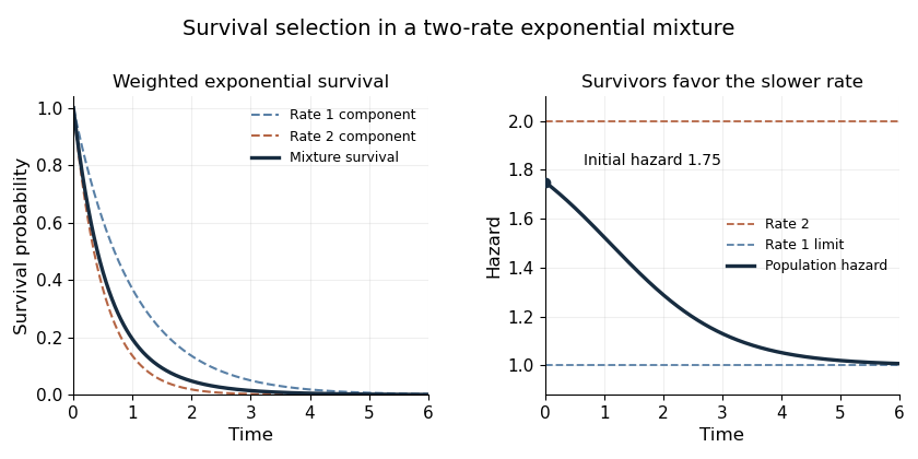
A frailty model uses an unobserved nonnegative random hazard multiplier to represent variation in individual risk. In a proportional frailty model, conditional on $U=u$ the cumulative hazard function is $u{H}_0(t)$, giving survivor $e^{-u{H}_0(t)}$. Averaging over the frailty random variable by the law of total probability yieldsthe Laplace transform of the frailty distribution evaluated at the baseline integrated hazard. This also applies to atoms by integration against the probability measure; the printed Dirac expression is not an ordinary continuous density.

In the given two-atom case, the Dirac delta function notation assigns probabilities $1/4$ and $3/4$ to $U=4/7$ and $U=8/7$. These have mean one, fixing the frailty scale relative to the baseline hazard. With $H_0(t)=7t/4$, the two conditional integrated hazards are $t$ and $2t$. ThereforeThe frailty distribution among survivors shifts toward the smaller multiplier $4/7$ over time, reproducing the declining population hazard and limit one without changing either individual's constant conditional hazard.