A tangent vector at is a derivation at a point: a real-linear map on germs of smooth functions satisfyingAddition and scalar multiplication preserve this identity, defining the tangent space as a vector space. A derivation annihilates constants. In a manifold chart centered near , the local factorization , with , gives . The factorization follows by integrating the first derivatives along a straight segment in a sufficiently small coordinate ball. ThereforeConversely these coordinate derivatives satisfy the derivation identity, so they really give a basis rather than merely a spanning family.
The cotangent space is the dual vector space . Its basis is characterized by . If , the chain rule gives the cotangent coordinate transitionThe cotangent bundle is the disjoint union , with projection . For each base manifold chart , defineIts inverse sends to . On overlaps the transition is , with the displayed fibre-linear transformation. Its coefficients and inverse are smooth, so these maps give a smooth atlas in dimension . Give the total space the topology obtained by transporting the product topology through these charts. Different base points are separated by disjoint base neighborhoods; distinct points over the same base point are separated within one bundle chart. A countable base smooth atlas and countable product bases give second countability. Thus the total space is a Hausdorff, second-countable smooth manifold. The same charts are vector bundle trivializations, since is product projection and their fibre changes are invertible linear maps.
The intrinsic canonical one-form on a cotangent bundle isIn the bundle chart it is . This definition is coordinate independent, hence its exterior derivative is the globally defined smooth differential two-formThis sign follows the fibre-first order in this problem; the equally common position-first symplectic form is . The volume formnever vanishes. A smooth manifold is orientable exactly when it admits a nowhere-zero top-degree form; its positive ordered bases determine a consistent orientation. Consequently is an orientable smooth manifold, even when is not. This is cotangent bundle orientation. In dimension zero the same conclusion uses the nowhere-zero zero-form .
A vector field is a smooth section of the tangent bundle. It differentiates smooth functions by . Define the Lie bracket of vector fields intrinsically byExpanding this expression on a product shows that the two mixed terms cancel, giving . It is therefore a derivation, hence a vector field. In local coordinates,Its coefficients are smooth. The intrinsic definition depends on no chart, which proves coordinate independence of this formula and defines the bracket on the whole manifold.
For a Lie group , let be Left translation on a Lie group. A left-invariant vector field satisfies for every . Evaluation is linear and injective, since . Conversely any gives a smooth left-invariant vector field . Smoothness follows from smooth multiplication and its differential. ThusFor any diffeomorphism , the intrinsic bracket identity on functions gives . Applying this naturality of the Lie bracket to proves that the bracket of two left-invariant vector fields remains left invariant. Evaluation at therefore defines the Lie algebra bracket on .
For the special orthogonal group, differentiation of at gives , so its tangent space is contained in the skew-symmetric matrices. Conversely, for any such , the matrix exponential satisfies and lies in the determinant-one component, because and its determinant varies continuously in . Its initial derivative is , provingFor matrices, . Extend these fields to the open matrix group , where the differential of in direction is . HenceRestriction to the embedded special orthogonal group preserves this bracket because the fields are tangent. Evaluating at gives , the required bracket on the Special orthogonal Lie algebra. The commutator is again skew symmetric. This calculation is differentiating left-invariant matrix fields; reversing the order of the two differentials would give the wrong sign.
Let have rank . A vector bundle covariant derivative is a real-linear operatorPairing its one-form slot with a vector field gives , with and .
In the horizontal description, a connection on a vector bundle is a smooth splitting , where , and the horizontal choice is compatible with fibre addition and scalar multiplication. This linearity is essential; an arbitrary nonlinear horizontal splitting is not a vector-bundle connection. Identify a vertical vector at with the element of obtained by differentiating the curve . Let be vertical projection followed by this identification. The induced vector bundle covariant derivative isIn a local frame of a vector bundle , a linear horizontal splitting has the formfor a matrix-valued connection one-form . Thus for , , which directly verifies the Leibniz rule.
Conversely, the Leibniz rule makes local: if a section vanishes near a point, multiply it by a smooth cutoff function supported in that neighborhood and equal to one near the point to see that its derivative vanishes there too. Local sections can therefore be differentiated by any extension agreeing near the point. Given , define its local connection one-form by . The Leibniz rule gives . Under , , one hasThe tangent fibre coordinate transforms by , so transforms precisely to . Consequently these local horizontal subspaces of a vector bundle connection glue to a smooth linear splitting inducing the given . Its local formula also shows uniqueness. This proves the horizontal connection associated to a covariant derivative construction.
A horizontal lift of is a smooth curve in with and . In a local frame write . Horizontality is exactly the linear ordinary differential equationWe use existence and uniqueness for an ODE with smooth coefficients, and the continuation theorem that a solution extends across a finite interval when it remains bounded inside the coordinate domain. For a linear system with continuous coefficients bounded by on a compact time interval, the Gronwall inequality bounds by its initial norm times , preventing finite-time fibre escape. Cover a compact subinterval of by finitely many bundle charts and partition it so each piece lies in one chart. Solve successively, changing fibre frames at the partition points. Coordinate invariance of the horizontal equation and uniqueness make the pieces agree. Exhausting by compact intervals containing produces a unique horizontal lift on all of for every prescribed . This is global continuation of linear parallel transport.
The lift equation is linear in its initial value. Hence the endpoint map is linear. Solving the same equation backwards, or transporting along , gives its inverse, soThis is parallel transport. For two parallel lifts , the assumed metric connection identity extends along the embedded curve and becomesHere is the covariant derivative along a curve. The permitted extension of sections and the tangent vector along the embedded curve justifies applying the bundle identity; equivalently it follows in each local frame. Thereforeso parallel transport is an isometry. This is the principle that parallel transport preserves a fibre metric.
Write for the Levi-Civita connection and define its Christoffel symbols by . For the Riemannian metric matrix and its inverse ,A curve with affine parameter is a geodesic when , equivalentlyThe connection is metric compatible and torsion free; in particular . The coordinate velocities are , and the displayed coefficients are smooth functions of position.
For whose initial-value geodesic exists through time , with and , define . The domain is open and contains a neighborhood of zero. Indeed the geodesic equation is a smooth first-order ODE in ; the constant solution with initial velocity zero exists through time , and existence on a compact time interval and smooth dependence persist for nearby initial data. Reparameterization and uniqueness give wherever defined. Consequently the differential of the exponential map at zero isThe inverse function theorem gives a neighborhood of zero on which is a diffeomorphism onto a neighborhood of . Shrink to a ball in and choose an orthonormal basis there. Its linear coordinate functions composed with are the geodesic normal coordinates on . This establishes well-defined local coordinates without assuming geodesic completeness.
In these geodesic normal coordinates, every radial geodesic has coordinate expression . Its equation at reads for every . The coefficients are symmetric in by the torsion-free connection property. Evaluating at the coordinate unit vectors and their pairwise sums, or using the polarization identity, therefore givesThis is the fact that Christoffel symbols vanish at the center of normal coordinates. Also , since is the identity in an orthonormal basis.
For sufficiently small , the geodesic sphere is . It is a smooth hypersurface because is a diffeomorphism on the ball. It equals the local distance sphere for sufficiently small radius, as the length comparison below shows; no assertion of global smoothness for large radii is needed.
The full Gauss lemma isfor in a star-shaped domain of and . To prove it, set , and , for near zero. Every -curve is a geodesic and has squared speed . The torsion-free connection property and the commuting parameter fields give ; metric compatibility and then giveAt , , so . Integration from to followed by setting proves the boxed identity, because and . For any in the domain, a small neighborhood of its compact radial segment suffices for the variation. The zero vector is covered directly.
In particular, if , the images of the radial and spherical tangent directions are orthogonal; taking also proves preservation of radial length. Thus in geodesic polar coordinates the Riemannian metric has radial part and no mixed radial-angular term. Every curve in a small normal ball from its center to radial coordinate has length at least , by integrating the absolute radial derivative; the radial geodesic realizes this length. To exclude shortcuts leaving the ball, choose a larger normal ball of radius with compact closure in and restrict to : an escaping curve first reaches radial coordinate and already has length at least . This proves the asserted small-radius distance interpretation and orthogonality of radial geodesics to geodesic spheres.
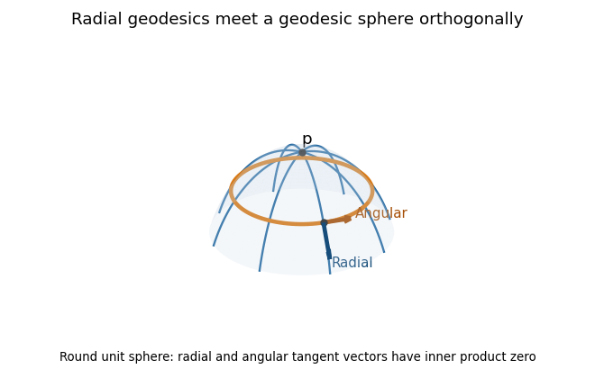
Radial geodesics and a geodesic sphere on the round unit sphere, with orthogonal radial and angular tangent vectors
. Details. 
Use real differential forms and the usual convention that a smooth manifold has no boundary unless one is specified. On a noncompact manifold the formal-adjoint identity below uses compactly supported forms. On a compact manifold it has no boundary contribution; if a boundary were allowed, extra boundary conditions would be necessary.
The Riemannian metric gives the dual inner product on and hence the inner product on exterior powers of a cotangent space:Extend this bilinearly. Equivalently, the increasing wedge products of an orthonormal coframe are an orthonormal basis of . The Hodge star operator is the unique map satisfying . If is a positively oriented orthonormal coframe, . Moving the factors of across the factors of its complement changes the sign by , soThe basis formula also proves that is an isometry.
For and with compactly supported product, the Stokes theorem and the Leibniz rule for the exterior derivative giveThus . The formal adjoint operator satisfies . Applying the inverse star and its square on degree gives the codifferentialThe exponent is congruent to modulo two, so this convention is consistent in every degree. Define the Hodge Laplacian by and a harmonic differential form by . On a compact manifold,Both nonnegative terms vanish for a harmonic form, giving . Conversely these two equations imply harmonicity.
Now let . The printed eigenvalue relation omits the subscript on its right-hand side; the intended equation is . On two-forms , soThese are respectively self-dual two-forms and anti-self-dual two-forms, and sum to . Their uniqueness follows because the and eigenspaces have zero intersection. Star is an orthogonal involution here, hence is self-adjoint and its opposite eigenspaces are orthogonal.
For closed two-forms define . Adding to changes the integral by ; adding an exact form to has the same effect. This is the real de Rham intersection form in dimension four. The wedge product of differential forms in degrees two and two is symmetric because ; hence is a symmetric bilinear form on .
In four dimensions in every degree. If is a harmonic two-form, gives , and gives . Thus is harmonic, and is the harmonic star-eigenspace decomposition. Use the permitted unique harmonic representative for each de Rham cohomology class. For harmonic ,The mixed terms vanish by orthogonality. The first restriction is positive definite and the second negative definite. In particular a nonzero harmonic has , proving nondegeneracy. Hence the signature of the intersection form from harmonic duality isThe finite dimensions and the harmonic description also follow from the Hodge decomposition theorem.
For completeness, the Hodge decomposition theorem on a compact oriented Riemannian manifold without boundary states the finite-dimensional harmonic space and the -orthogonal direct sumThe three summand components are unique, although their potentials need not be. Given an exact three-form on , decompose its smooth two-form potential as , with . Since and , . Put . In dimension four, , and on two-forms gives , so . ConsequentlyThis constructs a self-dual primitive of an exact three-form. The sum contains no factor : it is twice the self-dual projection of the coexact potential. Using the unscaled projection alone would give . This proves the final unheaded request.
Articles by others on the same topic
There are currently no matching articles.