Put . Conservation of specific orbital energy and specific angular momentum givesThe last comet expression is the vis-viva equation at the planet's orbit. The planet has only tangential velocity, while the comet's tangential component is . Consequently its prograde relative velocity is exactly, before planetary deflection,In the near-parabolic encounter limit , this reduces toThe displayed approximation also requires . The assumptions and alone do not guarantee it: an orbit with encounters the planet near apoapsis and has , not .
If all coplanar near-parabolic planet-crossing comets are admitted, so that , the tangential component ranges from to when retrograde orbits are included. ThusFor prograde orbits alone the upper limit is ; for the stated deep-crossing limit , both prograde and retrograde encounters approach . These are the speeds outside the planet's gravitational well. The surface impact speed is , where is the planetary escape velocity; under negligible gravitational focusing the two speeds agree.
For an unperturbed Kepler orbit, successive revolutions advance the planet-relative orientation by modulo , where is the comet's orbital period. An irrational period ratio makes these orientations dense; sufficiently distant mean-motion resonance and adequate observation time justify the corresponding phase mixing approximation.
At each radius between its pericentre distance and apocentre distance, the comet eventually visits every azimuth in the rotating reference frame. The spatial projection is thereforeIt is an annulus, with a nonuniform radial residence probability, rather than a uniformly filled area. Strictly, the full position-velocity phase space is not this annulus: at each radius the energy and angular momentum constrain the velocity, with inward and outward branches. The annulus is its position-space projection. This description assumes the orbital elements have not yet been substantially changed by planetary scattering.
The radial velocity of a Kepler orbit follows from the vis-viva equation after subtracting the tangential component:Each radial interval is crossed twice per orbital period, so its fraction of time isThis is the phase-mixed radial probability of a Kepler orbit, normalized to one between and . Dividing by the annular area gives the phase-mixed comet surface density per comet:For ,The printed density has the powers of and interchanged. Its expression is too large by in this limit. The normalized residence-time derivation fixes the corrected expression, which is also required for the later ejection-time scaling. For a population of independent identical comets, multiply by to obtain a number surface density of a disk.
With negligible comet radius and mass, the planet's radius and escape velocity areGravitational focusing changes the limiting collision impact parameter from to . Thus it is negligible when .
Put and in the prograde approximation. Substituting givesEquivalently . For , use . If negligible gravitational focusing is required for every coplanar near-parabolic orbit, including nearly tangential prograde encounters, use the smaller value .
A coplanar target sweeps a strip of width through the comet's local position probability. Hence the relevant geometric collision cross-section is a length, and the rare collision rate per comet is .
Using the corrected phase-mixed comet surface density and the notation , , the coplanar comet collision time isFor , this becomes , so at fixed stellar mass and planetary mass density. This is the mean waiting time for one orbiting comet; the mean interval between impacts from such independent comets is . It assumes rare encounters and orbital phase mixing, not a Poisson process derived from a single deterministic trajectory.
Suppose the inclined population samples its arguments of periapsis and nodal orientations, or that sufficiently slow precession supplies this sampling. Near the planet the vertical amplitude is . For uniformly distributed vertical phase, has probability density function , so the midplane volume probability is .
In the genuinely three-dimensional regime , the geometric collision cross-section is . The relative velocity differs from the coplanar value only at order for the specified high-speed encounters. Therefore the inclined comet collision time isAt fixed the leading scaling is , with no leading dependence when . The displayed factor retains the first dependence on . Also in this averaging convention.
Inclination alone does not specify a collision time for one fixed orbit. If its orbital nodes miss the planet's orbit, a tilted Kepler orbit can have no collisions at all. The finite result is an orientation-averaged population result, or requires precession or scattering to sample those orientations. When , the three-dimensional estimate crosses over to the coplanar result instead of tending to zero.
In a planetary gravitational assist, the incoming and outgoing relative speeds have the same magnitude. If is the planet-frame velocity, the heliocentric specific orbital energy change is consequentlynot an arbitrary addition of to the heliocentric speed. The initial binding energy per unit mass is .
For a weak deflection, , the hyperbolic scattering formula gives . Its direction is perpendicular to the incoming relative velocity. At the planet, in the near-parabolic prograde limit,On the favorable side of the planet the energy gain is approximately . Equating this to the binding energy gives the ejection impact parameterOnly one sign of impact parameter gains energy for each radial branch. Noncolliding ejections have , giving width , where . For , the planetary ejection of a comet rate is approximately . With this givesThe scaling applies when so that the local two-body encounter and weak-deflection approximations are consistent. The favorable-side coefficient assumes a coplanar orbit; averaging over other encounter geometries changes it. Cumulative diffusion by many subthreshold encounters is not included in this one-encounter estimate.
Exclude collisions from the ejection count. The effective collision width is , while the favorable noncolliding ejection width is . Define the first flyby-ejection threshold and the equal-rate crossover byThere are no direct noncolliding ejections in this weak-deflection model for . Above that threshold, comparison of the two rates gives collision is more likely for , while ejection is more likely for . In the deep-crossing limit , so its scaling at fixed density is . Order-one factors depend on encounter geometry; the robust condition compares with .
Adding the mutually exclusive rare-event loss rates gives the collision-ejection lifetime of a comet:For this is . For it approaches . A logarithmic sketch therefore bends from slope to slope , with no maximum. At the equal-rate crossover the lifetime is half either individual loss time.


These asymptotic branches use the corrected residence density from part iii and require and a local encounter scale below the Hill radius. They cannot be extrapolated indefinitely to arbitrarily distant weakly bound orbits.
For , differentiate the logarithm of the proposed Poynting–Robertson drag invariant:Substitution of the orbit-averaged Poynting–Robertson drag rates gives, over the common denominator , the numerator . HenceEquivalently, eliminating time gives , whose integral is . An exactly circular orbit remains circular; the expression for is singular at and is replaced by that separate solution.
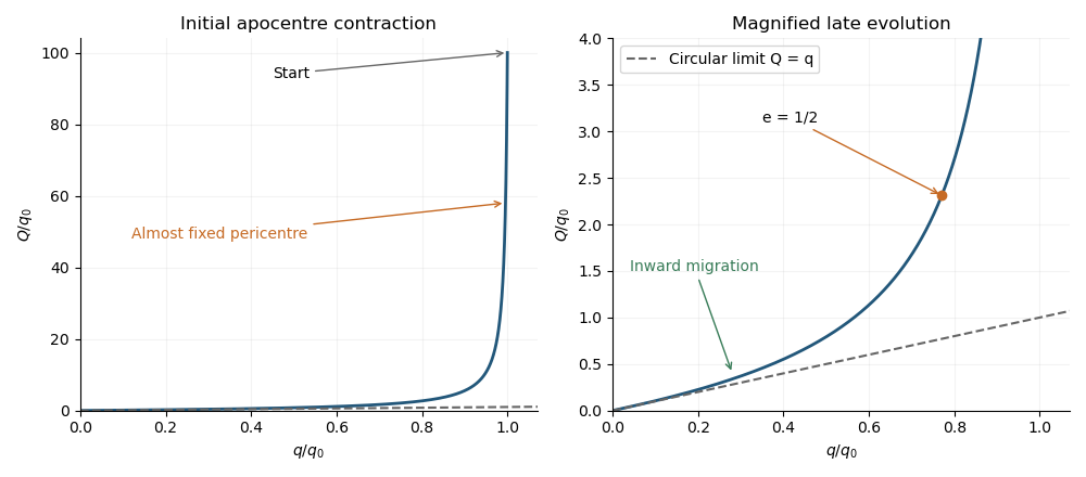
Using and , differentiate each apsidal distance. The apsidal evolution under Poynting–Robertson drag isBoth the pericentre distance and apocentre distance decrease. Since and , the same rates areTheir ratio isIn particular gives , whereas the circular limit gives slope .
Parameterize the trajectory by the decreasing orbital eccentricity. The Poynting–Robertson drag invariant givesFor , . Initially , and the orbit moves almost vertically down a plot of against : the apocentre distance shrinks rapidly while the pericentre distance changes little. Integrating the high-eccentricity slope givesOnce the orbit has moderate orbital eccentricity, both distances change appreciably. For example gives and in the limit. Eventually , , and the trajectory approaches the diagonal before reaching the origin. Thus the two approximate phases are apocentre contraction at nearly fixed pericentre, followed by nearly circular inward migration. They are a smooth crossover, not two separate exact solutions.

For a circular Kepler orbit, remains an exact solution of the averaged Poynting–Robertson drag equations, and . Integrating gives , so the point-star inspiral time under Poynting–Robertson drag isFor a star of radius , contact occurs instead at within this model. Sublimation or other forces can remove a real grain earlier.
Eliminate using the Poynting–Robertson drag invariant, . The eccentricity rate becomesSince the point-star limit corresponds to and , the inspiral time under Poynting–Robertson drag isFor , the integral is , recovering despite the apparent singularity of .
For , use and . The endpoint asymptotic integral is , givingMost of this long lifetime is spent near the initially large apocentre distance, before substantial circularization. The result assumes weak drag and a valid orbital average; near-parabolic release can violate that assumption.
Assume negligible fragment release speed relative to a circular parent planetesimal. Its initial speed is , but radiation pressure reduces the grain's gravitational parameter to . Its specific orbital energy and specific angular momentum areFor , the resulting dust orbit released from a circular parent ring hasRelease is at periapsis: the inherited tangential speed exceeds the new circular speed. Low- grains remain near the dust birth ring; higher bound gives increasingly eccentric orbits extending well outside it. Uniform release longitude produces an approximately axisymmetric dust halo, with long residence times near apoapsis. At the conservative release orbit is parabolic; above this radiation-pressure blowout threshold it is initially unbound. For , zero or repulsive effective gravity also prevents a bound ellipse.
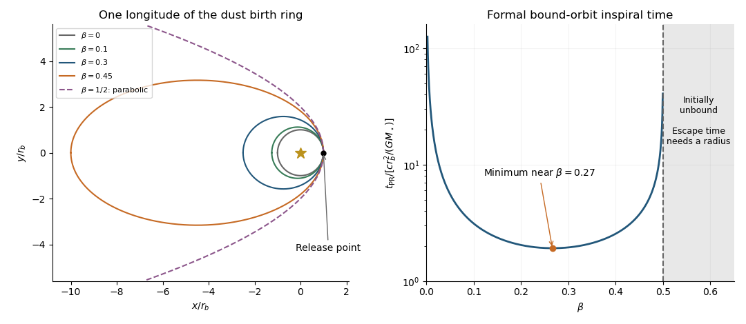
Dust release orbits and inspiral time under Poynting–Robertson drag
. Left: representative orbits released at one point on the birth ring, including the parabolic release limit. Right: the formal averaged lifetime of bound grains as a function of the radiation-pressure coefficient. Details.
The left panel shows one release longitude; rotating it around the ring fills the halo. At longer times Poynting–Robertson drag also carries bound grains inward, so an initially outward-spanning release distribution does not imply an empty inner region in a continuously supplied, collision-free population.
For the bound release orbits, use andThe inspiral time under Poynting–Robertson drag is thenThe limiting branches areThus the formal bound-grain curve, shown in the right panel of the preceding figure, diverges at both ends and has a minimum at an intermediate . At there is no Poynting–Robertson drag and the circular grain survives indefinitely in this collision-free model.
Initially unbound grains do not have a bound-orbit inspiral lifetime. For the release calculation gives outward trajectories; their residence time in a specified finite observation region is a dynamical escape time, not the averaged above. A numerical escape lifetime cannot be assigned without specifying the outer boundary. Extremely close to , energy lost on the first passage can alter even this bound/unbound classification: orbital averaging requires roughly . Accordingly the divergence is a formal limit of the supplied secular equations, not an exact prediction for marginal grains.
Differentiating the disturbing function in Lagrange planetary equations givesFor the complex eccentricity ,Use . Each planetary term becomes , soUnlike the polar orbital element equations, this linear equation is nonsingular at .
The planetary expansion is a decomposition into secular eigenmodes of conservative linear Laplace-Lagrange secular theory. It assumes small orbital eccentricities, coplanarity, approximately constant semi-major axis values, and averaging over fast orbital phases away from important mean-motion resonances and close encounters. Dissipation, migration, and nonlinear secular effects are absent from this constant-coefficient representation.
The are real eigenfrequencies of the Laplace-Lagrange secular matrix, describing apsidal precession. For mode , the signed real coefficients give its amplitude in planet ; their relative magnitudes are fixed by an eigenvector, and their signs distinguish aligned and anti-aligned apsides. The common phase specifies that mode's orientation at the chosen time origin. A planet's actual orbital eccentricity is , which generally varies through interference of modes; it is not a sum of the positive mode amplitudes.
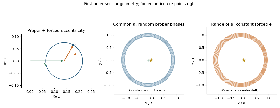
Put . For , the solution of the linear secular forcing of a test particle equation isThe initial condition gives and . The proper eccentricity is the constant amplitude of the homogeneous response; its proper longitude of periapsis is . The forced eccentricity is the driven vector , not necessarily a constant magnitude.
On an Argand diagram, describes a circle of radius . Its center can itself move under the planetary modes, so need not trace one fixed circle in the inertial complex plane. At a secular resonance , that mode instead produces , and the undamped linear response grows until the approximation fails.

For one isolated perturbing planet, its Kepler orbit has fixed longitude of periapsis, so is constant and its secular forcing frequency is zero. A constant forced eccentricity satisfies . Since ,This assumes . If an external process made the planet precess at frequency , the particular solution would instead be ; the stated formula relies on the isolated single-planet case.
To first order in orbital eccentricity, the semi-minor axis is , while the ellipse's center is displaced from the star by . Thus each orbit is a circle of radius about , in complex spatial coordinates.
Write at one secular epoch. The centers of the individual circles lie on a circle of radius about . Their union is the proper-eccentricity annulusIts full radial width is and its center is displaced by toward the forced apoapsis direction. Relative to the star, if the forced longitude of periapsis is zero,The middle panel of the preceding figure shows this construction. For fully sampled orbital phases and proper phases, the annulus is occupied throughout, but its density need not be uniform; turning points in the proper radial excursion give integrable edge enhancements. The construction requires and is an instantaneous secular geometry.
If the proper eccentricity is negligible and the semi-major axis ranges over , particles lie on nearly aligned forced Kepler orbits. For a locally constant forced vector, these are geometrically similar ellipses, represented to first order by circles of radius centered at .
The boundaries of the aligned eccentric ring are thereforeIt is narrower at forced periapsis and wider at forced apoapsis, unlike the constant-width proper-eccentricity annulus. Its centers shift slightly between the two edges, as shown in the right panel of the figure. The condition makes the proper radial excursion negligible compared with the variation in forced center location.
The forced vector need not actually be constant across the interval. More generallyFor aligned apsides this becomes , provided the orbits remain nested. The radial gradient of forced eccentricity matters for the density comparison even in a narrow ring.
For a phase-mixed orbit, probability in a short arc is , so the line density on a Kepler orbit is inversely proportional to speed. At true anomaly ,Using the vis-viva equation, and hence . ThereforeFor one particle, the normalized line probability is . This is density per arc length; density per unit polar angle has a further factor and is proportional to .
In the proper-eccentricity annulus, averaging over random proper phases cancels the proper vector in the first-order angular variation. The mean line density is proportional to , while the full ring width is independent of angle. Thus at corresponding radial locationsThere is a forced-apocentre enhancement in number surface density of a disk, together with the proper-excursion edge profile.
For a narrow aligned eccentric ring with locally constant , its width has the same first-order factor as its line density. Their ratio is constant: the constant-eccentricity aligned ring has no first-order surface-density contrast. It still contains more particles per unit longitude at apoapsis, spread across a wider area.
The more general surface density contrast in an eccentric ring depends on the eccentricity gradient. With a smooth number distribution per unit semi-major axis and aligned apsides,Hence decreasing can also make the aligned ring apocentre-dense; for it has the same first-order contrast as the proper-phase case. A positive gradient gives a pericentre enhancement. The problem leaves this profile unspecified, so there is no universal observational distinction based solely on the two apse densities.
Resolved ring width and a measured forced-eccentricity profile can distinguish the constant-width and similar-ellipse constructions. Interpreting observed brightness additionally requires the grain temperature, illumination, emissivity, and viewing geometry; brightness is not itself particle number density. Inferences from one contrast alone can therefore be degenerate.
Measure angles from periapsis in the direction of motion. The true anomaly is the angle at the stellar focus between the pericentre ray and the star-particle radius vector. Draw the auxiliary circle of radius around the ellipse's center; the point on that circle with the same projected major-axis coordinate as the particle defines the eccentric anomaly at the center.
The mean anomaly is a uniformly advancing time phase, with at pericentre passage . It is the angle swept by a fictitious uniformly moving circular phase marker, not generally the actual position angle. The mean motion is the angular frequencyThe second formula is Kepler's equation, which converts the uniform time phase into geometric position.
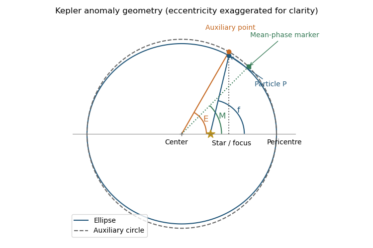

With the ellipse center as origin and its major axis horizontal, the auxiliary-circle construction gives particle coordinates , , while the stellar focus is at . ThereforeSquaring and adding gives . The Kepler orbit radius and the anomaly conversion are consequentlyEquivalently,The sine and cosine formulas, or a quadrant-aware angle function, fix the correct branch when using the half-angle relation.
Iterating Kepler's equation once gives . The exact radius expression then yieldsExpansion of the true anomaly conversion gives , soThe factor of two includes both the nonuniform relation between and and the change from center angle to focus angle .
Choose the common initial longitude of the particle and as zero. Let the fixed inertial longitude of periapsis be , positive ahead of that ray. At release , but the mean anomaly isThereafter , , and the particle's longitude is . The reference ray has longitude .
In the rotating reference frame, the radial axis points outward along the star- ray and the axis points forward. Define . The exact positional relations are
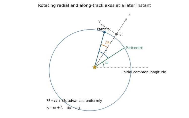

The diagram shows a later instant; initially , so . Retaining the correction in is what will preserve that initial condition in the approximate trajectory.
To first order, the initial-phase correction in can be omitted inside a term already multiplied by . ThusFor and , expand the exact rotating reference frame coordinates. Products of the small radial and angular displacements are second order. This givesAt the two sine terms cancel, as required. Equal mean motion gives a closed local epicyclic motion with radial-to-tangential amplitude ratio ; unequal mean motion adds along-track drift. The local expansion also requires , so small frequency mismatch alone does not justify it for arbitrarily large times.
Write and . The leading Keplerian shear isThe distinction between total mass and the individual planet's two-body central mass is order , below the retained order .
At one common reference epoch, the local Kepler orbit expansion takes the formwhere is the initial mean longitude relative to the rotating reference ray. Comparing its sine and cosine coefficients with the free solution of Hill equations givesThe required orbital elements from Hill coordinates are thereforeThese equalities have the first-order accuracy of the local approximation. If , the longitude of periapsis is undefined. The combination fixes the initial true longitude divided by . The special initial alignment imposed in part v would require , but the general two-planet solution need not impose it.
Substitution also verifies and : these are the unforced Hill equations. Close encounters add mutual-gravity forcing and can change the constants. Replacing by in the oscillation is consistent at leading order over local orbital times; accumulated phase differences must be retained when following much longer evolution.
Articles by others on the same topic
There are currently no matching articles.