Past exam of the mathematics course of the year 2 of the natural sciences course of the University of Cambridge / 2006 / Paper 1

In Cartesian coordinates, $\nabla \Phi =({\Phi }_x,{\Phi }_y,{\Phi }_z)$. For orthogonal coordinates, let $\mathbf{r}(q_1,q_2,q_3)$ be the position, $h_i=|\partial \mathbf{r}/\partial q_i|$ the scale factors of orthogonal coordinates, and ${\mathbf{e}}_i=h_i^{-1}\partial \mathbf{r}/\partial q_i$ the corresponding unit vectors. Since $d\mathbf{r}={\sum }_i{h}_i{\mathbf{e}}_{i}d{q}_i$ and $d\Phi =\nabla \Phi \cdot d\mathbf{r}={\sum }_i{\Phi }_{q_i}d{q}_i$, comparison of independent increments gives the gradient in orthogonal coordinates:For the hyperbolic parametrization of oblate spheroidal coordinates, the three coordinate tangent vectors areTheir pairwise dot products are zero. Their squared Euclidean norms are ${\sinh }^{2}R+{\sin }^2\theta$, ${\sinh }^{2}R+{\sin }^2\theta$, and ${\cosh }^{2}R{\cos }^2\theta$, respectively. Thus the coordinate surfaces meet orthogonally wherever this is a regular coordinate chart, andThe last expression uses the usual latitude range $|\theta |<\pi /2$; without that range a scale factor is its absolute value. Axial or ring degeneracies are excluded from a regular chart.

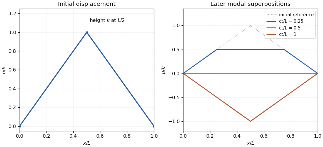
Separation of variables in the wave equation with fixed endpoints selects $H_n(x)=\sin (n\pi x/L)$ and angular frequencies ${\omega }_n=cn\pi /L$, $n\ge 1$. The time factors may be chosen as $F_n(t)=\cos {\omega }_{n}t$, $G_n(t)=\sin {\omega }_{n}t$. By Fourier sine series orthogonality, the initial data giveHence $u={\sum }_{n\ge 1}[a_n\cos {\omega }_{n}t+b_n\sin {\omega }_{n}t]\sin (n\pi x/L)$. The factor $1/{\omega }_n$ in $b_n$ is required because differentiating the time sine supplies ${\omega }_n$.

The given displacement is a symmetric triangular tent: it is zero at both endpoints and has height $k$ at $L/2$. Integrating each linear half gives $a_n=8k\sin (n\pi /2)/(n^2{\pi }^2)$. Release from rest gives $b_n=0$, so the midpoint-plucked fixed-end string isOnly odd modes occur, by symmetry about the midpoint. The initial slope corner makes this a finite-energy weak solution; it is a classical solution away from the propagating corner lines.

With the stated angular-frequency convention, the inverse Fourier transform is $f(x)=(2\pi {)}^{-1}{\int }_{-\infty }^{\infty }\tilde{f}(k)e^{ikx}dk$. Direct integration gives ${\tilde{f}}_0(k)={\int }_0^{\infty }{e}^{-(\alpha +ik)x}dx=1/(\alpha +ik)$. For $n\ge 1$, integration by parts has zero boundary terms and gives ${\tilde{f}}_n=n{\tilde{f}}_{n-1}/(\alpha +ik)$. ThereforeThis also follows from the Fourier transform of a polynomial multiple, since multiplication by $x$ corresponds to $i{\partial }_k$.

To prove Parseval's identity, substitute the inverse transform of $g$ into $\int f^{\ast }g$. Under the assumed integrability, Fubini's theorem permits interchange, and the inner integral is $\int f(x{)}^{\ast }{e}^{ikx}dx=\tilde{f}(k{)}^{\ast }$. HenceApply this with $f=g=f_n$. The spatial Gamma integral is ${\int }_0^{\infty }{x}^{2n}{e}^{-2\alpha x}dx=(2n)!/(2\alpha {)}^{2n+1}$. The transformed squared modulus is $(n!{)}^2/({\alpha }^2+k^2{)}^{n+1}$, giving the scaled even rational Parseval integral

Decompose ${\mathbb{R}}^n=\mathrm{span}\{a\}\oplus a^{\perp }$. The rank-one matrix update $a{a}^T$ acts as multiplication by $\Vert a{\Vert }^2$ along $a$ and as zero on its orthogonal complement. ThusThe perpendicular eigenvalue has multiplicity $n-1$ and is absent when $n=1$. Consequently $A^{+}$ is always an invertible matrix, while

Put $\beta =\Vert b\Vert >0$ and choose an oriented orthonormal basis with third vector $b/\beta$. The Levi-Civita symbol term has action ${ϵ}_{ijk}{b}_k{x}_j=x\times b$, the negative of $b\times x$. Thus this axisymmetric linear map has block formThe transverse eigenvalues $1\pm i\beta$ are not real. The only real eigenvalue and its eigenvectors are thereforeThe determinants are $\det B^{+}=(1+{\beta }^2{)}^2>0$ and $\det B^{-}=(1-{\beta }^2)(1+{\beta }^2)$, proving that $B^{+}$ is always invertible, and $B^{-}$ is invertible exactly when $\Vert b\Vert \ne 1$. The complex transverse pair is important for this determinant even though the question asks for real eigenvalues.

A matrix is diagonalizable if some invertible $S$ makes $S^{-1}AS$ diagonal, equivalently if it has a basis of eigenvectors. If $A^p=0$ and $Av=\lambda v$ for $v\ne 0$, then $0=A^{p}v={\lambda }^{p}v$, so every eigenvalue is zero. There is at least one zero eigenvalue: otherwise $A$ and hence $A^p$ would be invertible. A diagonalizable nilpotent matrix has an all-zero diagonal form and therefore is zero itself.

For the specified matrices, direct determinant expansion givesThe Cayley-Hamilton theorem gives $B^3=0$. Its entry $B_{12}=-2$ is nonzero for every real $\alpha$, so $B$ is not diagonalizable for any $\alpha$. The matrix $C$ has three distinct real eigenvalues and is therefore diagonalizable over $\mathbb{R}$. For an explicit check, take columns $(-1,0,1{)}^T$, $(2,-3,1{)}^T$, $(2,3,1{)}^T$ in $S$; then $S^{-1}CS=\mathrm{diag}(-6,0,6)$.

For the normalized second-order equation $y^{\prime \prime }+P(x)y^{\prime }+Q(x)y=0$, an ordinary point has analytic $P,Q$. A regular singular point is a singular point where $(x-x_0)P$ and $(x-x_0{)}^{2}Q$ extend analytically through $x_0$. The two finite singular points here are $0$ and $1/2$. At zero, the respective limiting coefficients are $1/2,0$; at $1/2$, they are $-1,0$. Thus both are regular singular points, with indicial roots $0,1/2$ and $0,2$, respectively.

Use the Frobenius method and write $y=x^r{\sum }_{n\ge 0}{a}_n{x}^n$, $a_0\ne 0$, with coefficients at negative indices defined as zero. The lowest power gives the indicial equation $r(2r-1)=0$, so $r=0$ or $r=1/2$. Equating the coefficient of $x^{n+r-1}$ gives, for $n\ge 1$,For $r=0$ and $a_0=1$, the first coefficients are $1,2,2,4/3,\dots$. For $r=1/2$ they are $1,1,1/2,1/6,\dots$, multiplying $x^{1/2}$. The distinct nonintegrally separated indicial roots give two independent Frobenius series. The half-power solution is a generalized power series, rather than an ordinary Taylor series at zero.

The coefficients in the Taylor series areFor either series, the ratio test gives absolute term ratio $|x|/(n+1)$ or $2|x|/(n+1)$, tending to zero for each fixed real or complex $x$. Both have infinite radius of convergence.

Substituting $a_n=2^n/n!$ into the $r=0$ recurrence, and $a_n=1/n!$ into the $r=1/2$ recurrence, satisfies every coefficient equation. They give $e^{2x}$ and $\sqrt{x}{e}^x$. Thus on a positive interval not crossing a singular point,Their Wronskian is $e^{3x}(2x-1)/(2\sqrt{x})$, nonzero for $x>0$, $x\ne 1/2$, proving independence on each ordinary interval. Both functions are analytic near $1/2$, so this is an apparent regular singular point: a pole in normalized coefficients need not force a singular solution. The Wronskian can vanish at that singular point without making the two functions linearly dependent on an ordinary interval.

Multiply the original equation by $p(x)=\exp ({\int }^{x}u(s)ds)>0$. Since $p^{\prime }=up$, it becomes $(p{y}^{\prime }{)}^{\prime }+qy+\lambda ry=0$ with $q=pv$, $r=pw>0$. This is Sturm-Liouville form. For two real eigenfunctions, multiply the equation for $y_n$ by $y_m$, subtract the equation for $y_m$ multiplied by $y_n$, and integrate. The Lagrange identity for a Sturm-Liouville operator givesEach separated homogeneous boundary condition makes the corresponding determinant zero, provided its pair of coefficients is not both zero. For distinct eigenvalues, this proves the orthogonality of Sturm-Liouville eigenfunctions.

For the constant drift, the drift-removing substitution for a Dirichlet Sturm-Liouville problem is $y=e^{-\alpha x}v$. It reduces the equation to $v^{\prime \prime }+\lambda v=0$ with $v(0)=v(\pi )=0$. Nonzero solutions occur exactly atThe zero and negative values give only the zero solution under both endpoint conditions. The self-adjoint expression is $(e^{2\alpha x}{y}^{\prime }{)}^{\prime }+{\alpha }^2{e}^{2\alpha x}y+\lambda e^{2\alpha x}y=0$. Hence the weight is $r=e^{2\alpha x}$, and for the displayed normalization,

For the zero initial data, the Green function of an undamped oscillator is $G_0(x,s)=\sin [k(x-s)]/k$ for $0\le s\le x$, and zero for $s>x$. It is continuous at the source and its first derivative jumps by one. The resulting convolution isIt vanishes together with its first derivative at zero and has the required resonant forcing.

For the two-endpoint problem, write $L=\pi /(6k)$, $a=\min (0,L)$, $b=\max (0,L)$ and $\kappa =|k|$. This covers both signs of the supplied nonzero $k$. Left and right homogeneous solutions are $\sin [\kappa (x-a)]$ and $\sin [\kappa (b-x)]$, with Wronskian $-\kappa \sin [\kappa (b-a)]$. The Dirichlet Green function is thereforeIts endpoint values are zero and its first derivative jumps by one. Here $\kappa (b-a)=\pi /6$, so the denominator does not vanish. Integrating the constant forcing givesEquivalently $y=(1-\cos kx)/2+(\sqrt{3}/2-1)\sin kx$. The negative interior response is consistent with the negative kernel for this short Dirichlet interval.

Apply the Euler-Lagrange equation to the integrand of $F-\lambda G$, namely $p{y}^{\prime 2}-q{y}^2-\lambda r{y}^2$. With fixed zero endpoint values, it gives $(p{y}^{\prime }{)}^{\prime }+qy+\lambda ry=0$. Multiplying by $y$ and using integration by parts gives $F=\lambda G$, so each stationary Rayleigh quotient $F/G$ equals its eigenvalue.

In the half-line problem, $p=x$, $q=-x$, $r=1$, so the quotient is $R[y]={\int }_0^{\infty }x(y^{\prime 2}+y^2)dx/{\int }_0^{\infty }{y}^{2}dx$. For $y=e^{-\beta x}$, $\beta >0$, its numerator is $({\beta }^2+1)/(4{\beta }^2)$ and denominator $1/(2\beta )$. Hence $R=(\beta +{\beta }^{-1})/2$, minimized at $\beta =1$:For the compactly supported linear trial, $A>0$, the numerator is $A^2/2+A^4/12$ and denominator $A^3/3$. Thus $R=3/(2A)+A/4$, minimized at $A=\sqrt{6}$, givingThe derivative jump at the cutoff is allowed in the quadratic-form trial space of the Rayleigh-Ritz method: the trial is continuous and has finite form energy.

The exponential ground state of a linearly weighted Sturm-Liouville problem proves which estimate is best. Vanishing endpoint terms giveEquality occurs for $y=C{e}^{-x}$, which also satisfies the differential equation with $\lambda =1$. Thus the exponential trial gives the exact smallest eigenvalue, whereas the linear trial gives a larger upper bound. Finiteness at the singular endpoint supplies the regular branch with $xy{y}^{\prime }\to 0$; all the displayed trials have the required vanishing boundary terms.

For fixed endpoint values, stationarity requires the Euler-Lagrange equation $f_y-d(f_{y^{\prime }})/dx=0$. Differentiate $y^{\prime }{f}_{y^{\prime }}-f$ along an extremal: its derivative is $y^{\prime }[d(f_{y^{\prime }})/dx-f_y]-f_x$. Thus when $f_x=0$ the Beltrami identity makes that quantity constant.

Take $y$ as depth measured downward. Conservation of energy from rest gives $m{v}^2/2-mgy=0$, hence speed $v=\sqrt{2gy}$. With arc length $ds=\sqrt{1+y^{\prime 2}}dx$, the travel time is $T=(2g{)}^{-1/2}{\int }_0^{x_B}\sqrt{(1+y^{\prime 2})/y}dx$. For $f=\sqrt{(1+y^{\prime 2})/y}$, the Beltrami quantity is $-1/\sqrt{y(1+y^{\prime 2})}$. Thus $y(1+y^{\prime 2})=c>0$.

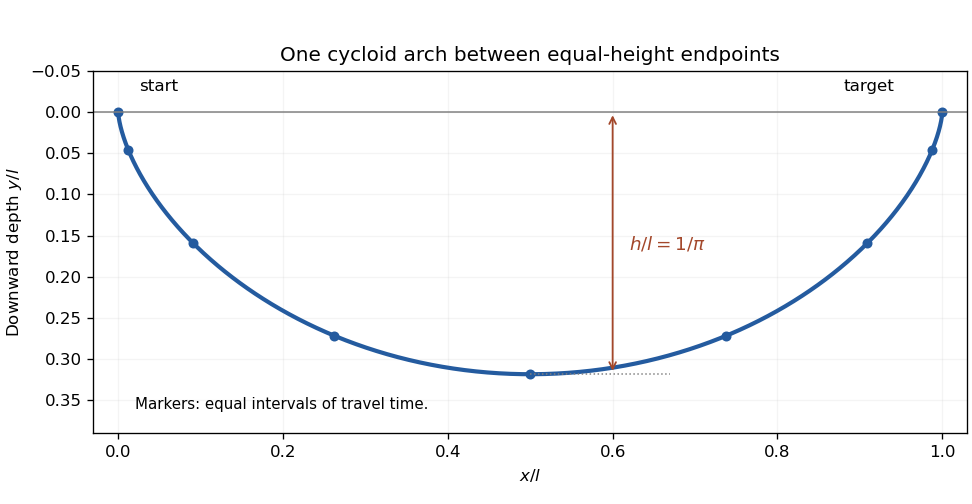
Put $y=c{\sin }^2\theta$ and take $y^{\prime }=\cot \theta$ along the first arch. Since $dy/d\theta =2c\sin \theta \cos \theta$, one obtains $dx/d\theta =2c{\sin }^2\theta$. Integrating from the initial cusp gives the cycloid solving the brachistochrone problem:For the equal-height target, the first complete arch has ${\theta }_B=\pi$, so $c=l/\pi$. Also $ds/d\theta =2c\sin \theta$ and $v=\sqrt{2gc}\sin \theta$ for $0<\theta <\pi$. ThereforeThe endpoint zeros of speed cancel the zeros of $ds/d\theta$, leaving finite travel time. Global minimality follows from the maximum-depth bound for a brachistochrone: any competing track with maximum depth $h$ satisfies $T\ge [l/\sqrt{h}+\pi \sqrt{h}]/\sqrt{2g}\ge \sqrt{2\pi l/g}$. The displayed cycloid attains both inequalities with $h=l/\pi$.