Treat each observed arrival label as a constraint on an unobserved walking duration. Departures are treated as fixed design information. Writing for the minutes available until work starts, the derived late-label thresholds have frequencies ; the early-label thresholds have frequencies . These are censoring thresholds, not measured journey times. A late label means , and an early label means ; equality has probability zero under the continuous model.
The paper specifies no prior distribution. One explicit proper model iswith independent priors; all times are in minutes. These ranges are a transparent modelling choice, not information deduced from the observations. In particular, this is a prior on the standard deviation , not a uniform prior on the variance . The normal distribution permits negative durations; it is the mathematical approximation requested here, rather than a claim that such durations are physically possible. A truncated model would be a different model.
The following Python implements hard conditioning by rejection sampling.
None marks a rejected trace; an accepted Boolean answers whether all five future arrivals are late. The same parameters are shared across past and future days.import math
import random
LATE = {20: 1, 21: 3, 25: 3, 27: 1, 32: 2}
EARLY = {29: 1, 34: 1, 36: 3, 37: 1, 38: 1, 39: 1, 43: 1, 44: 1}
RECORDS = [(c, True) for c, n in LATE.items() for _ in range(n)]
RECORDS += [(c, False) for c, n in EARLY.items() for _ in range(n)]
def journey_trace(rng):
mu = rng.uniform(0.0, 60.0)
sigma = rng.uniform(1.0, 20.0)
# Twenty latent past durations and five future durations.
past = [rng.gauss(mu, sigma) for _ in RECORDS]
future = [rng.gauss(mu, sigma) for _ in range(5)]
if not all(t > c if late else t < c
for t, (c, late) in zip(past, RECORDS)):
return None
return all(t > 30.0 for t in future)
def accepted_average(trace, n, rng):
if n <= 0:
raise ValueError("n must be positive")
successes = accepted = 0
while accepted < n:
result = trace(rng)
if result is not None:
accepted += 1
successes += int(result)
return successes / nFor example,
accepted_average(journey_trace, n, random.Random(2021)) estimates the desired conditional probability from accepted traces. Accepting False is essential: treating a false answer as a rejected trace would condition on the desired conclusion. The model deliberately emphasizes clear semantics; rejection can be inefficient because all twenty past-label constraints must hold together.An idealized underlying probability space iswith the product Borel sigma-algebra. Its 27 independent random coordinates are , , twenty past standard-normal noises, and five future standard-normal noises. Define . Sampling an unknown variance does not mean drawing a new variance on each day; a single draw of applies to all durations in a trace.
Let be the event that the first twenty durations satisfy their corresponding observed inequalities. The observations are the twenty late/early labels, conditional on the fixed departure thresholds. They are not exact values of the latent . The posterior probability measure on traces isHere : at every interior parameter pair each strict normal-tail probability lies in , so their finite product has positive prior integral.
The returned outcome isThus the underlying sample space has dimension 27, the successful output space is , and the observations define the conditioning event . The desired output probability distribution is the pushforward measure of under . Rejection is an implementation device, not a third scientific answer:
None is discarded before forming the conditional output law.Write for the standard normal distribution function. Integrating out the twenty independent past durations gives the threshold-censored normal likelihoodThe frequencies are those in part (a). For a future day, the conditional late-arrival probability is . Conditional independence of the five future durations gives .
Exactly three primitive random coordinates suffice. Draw from the same priors and one independent . Reject if ; otherwise return whether . Conditional on acceptance and the parameters, is uniform on an interval of length ; the true-answer subinterval has length . Reusing this same uniform value is therefore intentional, not an independence mistake.
Indeed the two output contributions at each parameter value areThese are exactly the contributions obtained by integrating the original twenty-five duration noises. Multiplication by the common prior density and normalization therefore give the same joint posterior distribution of . The revised program preserves the query and parameter posterior, but does not retain individual latent durations. This is uniform-interval encoding of conditioning and a binary query.
Here is an executable version, reusing the definitions from part (a). Logarithms avoid multiplying many small probabilities.
def normal_logcdf(z):
    value = 0.5 * math.erfc(-z / math.sqrt(2.0))
    return math.log(value) if value > 0.0 else -math.inf

def journey_loglik(mu, sigma):
    return (sum(n * normal_logcdf((mu - c) / sigma)
                for c, n in LATE.items())
            + sum(n * normal_logcdf((c - mu) / sigma)
                  for c, n in EARLY.items()))

def collapsed_trace(rng):
    mu = rng.uniform(0.0, 60.0)
    sigma = rng.uniform(1.0, 20.0)
    log_likelihood = journey_loglik(mu, sigma)
    # This uniform lies in (0, 1], avoiding log(0).
    log_u = math.log(1.0 - rng.random())
    if log_u >= log_likelihood:
        return None
    log_h = 5.0 * normal_logcdf((mu - 30.0) / sigma)
    return log_u < log_likelihood + log_h
accepted_average(collapsed_trace, n, rng) consequently has the same target as the original program. The ideal three-dimensional sample space is with product uniform probability measure, conditioned on the displayed acceptance event. Finite-precision normal tails can underflow to zero in this simple implementation; the mathematical equivalence concerns exact probabilities, and the numerical check in part (d) independently integrates the likelihood in the region carrying appreciable posterior mass.For any chosen proper prior density on with positive evidence, Bayes' theorem givesThe prior density comes from the first two random draws. The likelihood is the probability of satisfying all observed-label constraints after integrating the past duration noises. The factor is the probability of the five-day outcome conditional on the shared parameters. The denominator is the probability of acceptance, which converts the numerator's joint probability into the required conditional probability.
For the independent uniform priors in part (a), the constant cancels and both integrals reduce to , . A prior on the variance would require transforming the density: this chosen prior has density for conditional on . One must not silently replace it by a uniform prior on .
There is no unique numerical probability until the prior distribution is chosen. As a check for the stated uniform priors, independent Gaussian quadrature calculations with 256 and 512 nodes per coordinate agree at the shown precision:The prior-predictive probability of all observed labels is approximately , explaining the rejection cost. These numbers are illustrations of the explicit model, not additional observed data.
A subtle point is that the five future days are independent only conditional on . Integrating shared parameter uncertainty gives , not . The latter is about for these priors and understates the five-day probability. Jensen's inequality gives , while gives . For two future late-arrival indicator functions, their posterior covariance is . This is the posterior predictive repeated-success identity.
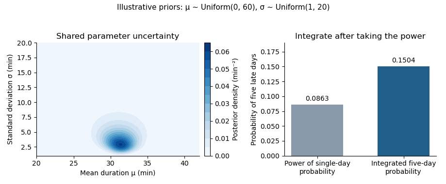
Posterior uncertainty and the five-day predictive probability for the explicitly chosen uniform priors. The contour is cropped to the parameter region carrying the visible mass; integration uses the full prior rectangle.
Details. 
I would first collapse the duration noises as in part (c), then use self-normalized importance sampling on the two shared parameters. Draw independent , give each the importance weight , and returnThis is likelihood weighting: the observations affect the weights rather than forcing repeated simulation of twenty latent inequalities. Integrating out both the constraints' auxiliary randomness and the future Boolean query is Rao-Blackwellization; at fixed parameters it removes randomness without changing the relevant conditional expectations.
The weights and weighted queries lie in , and the evidence is positive. The strong law of large numbers therefore makes the numerator and denominator averages converge to their corresponding integrals, proving almost sure convergence of their ratio to part (d). The finite- ratio is generally biased; the assertion concerns consistency rather than a finite-sample unbiased estimator. Use logarithms of importance weights to avoid numerical underflow:
def weighted_answer(n, rng):
    if n <= 0:
        raise ValueError("n must be positive")
    samples = []
    for _ in range(n):
        mu = rng.uniform(0.0, 60.0)
        sigma = rng.uniform(1.0, 20.0)
        samples.append((journey_loglik(mu, sigma),
                        math.exp(5.0 * normal_logcdf((mu - 30.0) / sigma))))
    offset = max(logw for logw, h in samples)
    if not math.isfinite(offset):
        raise ArithmeticError("all weights underflowed")
    scaled = [(math.exp(logw - offset), h) for logw, h in samples]
    den = math.fsum(w for w, h in scaled)
    answer = math.fsum(w * h for w, h in scaled) / den
    ess = den * den / math.fsum(w * w for w, h in scaled)
    return answer, ess
The returned effective sample size of importance sampling is a concentration diagnostic, not a proof of accuracy. Repeat runs and inspect the weights. If the prior is much broader than the posterior, improve the proposal with the corresponding importance sampling density correction, or use the Metropolis–Hastings algorithm targeting . Because this particular collapsed problem is only two-dimensional, deterministic numerical integration is also an excellent independent accuracy check; it was used for the figure and numerical illustration. Straight rejection of the original traces is correct but wastes most proposals here.
Articles by others on the same topic
There are currently no matching articles.