The scanned cover establishes Hilary Term 2018, despite the containing bundle's 2017 filename. Use , the Minkowski metric signature outside question 2, which uses Euclidean space, and . The phase and normalization conflicts in question 4 are identified in a; its path integral is evaluated with the normalization of its displayed action.
Divide the infinitesimal variation by its constant parameter , so the transformation generator is . The variation of the kinetic term isand that of is . Thus the Lagrangian density is invariant pointwise, without a nonzero boundary current. The finite transformation is a rotation of the two real scalar fields, giving an SO(2) global symmetry in field theory.
Noether's theorem supplies the parameter-independent Noether currentIts divergence is , since the first-derivative terms cancel. Both fields obey the same Klein-Gordon equation, so this vanishes on solutions. With spatial boundary conditions giving zero flux at infinity, the Noether charge isA finite box with periodic boundary conditions works as well. The spatial integral is conserved because the local continuity equation converts its time derivative into a boundary flux; neither vanishing local current nor constant individual fields is required. Equivalently, transforms as , exhibiting the equivalent global U(1) symmetry and fixing the sign of the generator.
The canonical momenta are , soDifferent species commute at equal times, so these products have no ordering ambiguity and is Hermitian. Write . Substituting the mode expansion of a free field and using the spatial Fourier transform identity givesSubtract the expression with species interchanged. The two-annihilator terms cancel after , as do the two-creator terms. Commuting different species in the remaining terms yieldsThere is no infinite vacuum contribution to the Noether charge to subtract: the contractions that would generate a species-diagonal constant are absent.
The bosonic canonical commutation relations giveDefine the creation operatorsTheir commutators with are . Since , the one-particle states haveThe fixed-momentum states are delta-function normalized; a square-integrable wave packet of either species is a normalizable state with the same Noether charge eigenvalue. In this basis , so it measures a difference of occupation numbers. The equal-time identity , independently checks the sign against a.
Take the free squared mass , as for the ordinary massive free theory. The quartic part of the scalar potential can be writtenIt is nonnegative for every real field value exactly whenNecessity follows from the axis and the diagonal : a negative coefficient on either ray makes tend to minus infinity under rescaling. The displayed sum proves sufficiency, since is also nonnegative. This is a copositive matrix condition on the quadratic form in the nonnegative variables , rather than positive definiteness on all independent signed variables.
The strict inequalities , make the quartic part grow in every nonzero direction. They are not necessary for a stable vacuum when . For example, gives two stable free massive fields; , has a flat quartic diagonal but a confining quadratic term. If , boundary cases have flat vacuum directions and need not have a unique isolated minimum. If one instead allows negative squared mass, a flat quartic ray makes the full potential unbounded below; the stability conditions must then be strengthened. This distinguishes boundedness from strict quartic coercivity.
Under the generator of a, the variation isIt vanishes identically if and only if . In that case preserves the entire global U(1) symmetry. More explicitly, the interacting Euler-Lagrange equations giveHenceA special solution lying on an axis does not establish an operator conservation law. Among the stable couplings, the symmetry-preserving line is .
Use mass dimensions with , and dimensionless action. The Lagrangian density in Euclidean space has dimension , and the kinetic term fixes . ThusA dimensionless coupling constant is thereforeHere is a positive regularization scale with mass dimension one. The interaction is marginal at its upper critical dimension , relevant below it and irrelevant above it by this engineering-dimension test. In particular, , while near . At this stage is the dimensionless version of the displayed bare coupling; after introducing counterterms one may use the same scale factor for the renormalized coupling.
Expand the normalized Euclidean path integral with weight and apply Wick's theorem. Use labelled external momenta and a fixed Fourier transform convention throughout. A line carrying momentum contributes . Each -valent interaction vertex contributes : its possible contractions cancel the factorial in the Lagrangian density. A vertex also carries with all incident momenta incoming. Integrate each independent loop momentum with and divide by the Feynman-diagram symmetry factor for fixed external labels. There are no Minkowski factors of .
For the full -point Green's function, include every graph in which all vertices belong to components attached to external insertions. In particular, disconnected components carrying external insertions must be included, and the zeroth-order result is the sum of free pairings. Pure vacuum bubbles cancel against the denominator. The connected Green's function restricts to connected graphs, while a one-particle-irreducible vertex imposes the stronger restriction that removing one internal line cannot disconnect the graph. These are different objects. Odd vanishes in the symmetric vacuum because every interaction has even valence. At fixed perturbative order, multiply by the appropriate power of the coupling and sum all allowed graph topologies and external attachments.
If the overall momentum-conservation delta function is removed by convention, report the remaining function as its coefficient. The ordinary unamputated Green's function includes external scalar propagators; dividing them out defines an amputated function. The definition in c performs this amputation but does not, by itself, impose the usual one-particle-irreducibility condition.
The single-vertex scalar two-point graph at first order in has one -valent interaction vertex. Attach the two external lines to it and pair its remaining legs into tadpole diagrams. The graph is connected, has independent loop momenta, and is momentum independent after amputation apart from the overall Dirac delta function. In particular, first order in the coupling need not mean one loop.
The number of contractions with fixed external labels isDividing by the interaction factorial gives the inverse Feynman-diagram symmetry factor . Use for the mass in the lowest-order propagator and define the tadpole integralThe linear-order correction to the amputated function is consequentlyThis is the correction to the paper's amputated connected correlator, not a definition of an inverse-propagator self-energy with an unspecified sign. At this order using instead of gives the same lowest-order integral.
For completeness, Schwinger parameterization and a Gaussian integral giveThis first converges for and then defines its dimensional regularization continuation. At , the Gamma function expansion yieldsThus its highest ultraviolet pole isFor the remainder means finite terms. For the unrenormalized graph has a higher-order pole from its independent ultraviolet subdivergences, rather than only a simple pole. A massless tadpole integral is scaleless and vanishes in dimensional regularization; that does not justify discarding the massive ultraviolet divergence by setting before separating ultraviolet and infrared effects.
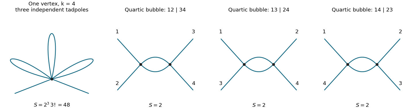
A single higher-valence vertex with three tadpole loops, and the three one-loop quartic bubble channels
. The first panel illustrates k=4; in general there are k minus one loops. The three remaining panels have identical topology and different labelled external attachments. Details.
The change of field and parameters separates the Lagrangian density in Euclidean space intoThe two-leg counterterm interaction vertex is , with the overall momentum conservation delta function understood. With , the explicit first-order contribution to the propagator isThe minus sign follows either from expanding or from expanding .
For , the loop correction is . Its ultraviolet pole from c isThere is no external dependence in the amputated tadpole diagram, so no one-loop wave-function renormalization is required. The minimal subtraction scheme therefore givesOnly the pole is subtracted: including would impose a different finite subtraction prescription. The defined is the coefficient in , not automatically the difference beyond this order.
Use the wave-function renormalization coefficient and anomalous dimension definition stipulated in this part, keeping their signs and normalization. Put . To the required order,At fixed bare , the leading change of the dimensionless coupling is , because has mass dimension . Therefore the chain rule, applied before setting , givesThusThe vanishing engineering contribution multiplies a pole and leaves a finite answer. Dropping it at the start would incorrectly give zero. The numerical answer is conditional on the supplied two-loop coefficient. A convention defining the field anomalous dimension as instead gives for the same ; substituting that convention silently would answer a different question.
A phi-fourth theory interaction has mass dimension , so its bare coefficient must contain a renormalization scale factor when expressed through a dimensionless renormalized coupling. The tree-level four-leg interaction vertex is linear in that coupling. At the next order, two quartic vertices form the three one-loop bubble diagram graphs shown in c, with external pairings , and .
For each pairing there are two identical internal lines and Feynman-diagram symmetry factor 2. The loop integral has the large-momentum behaviourIt is logarithmically divergent in four dimensions. Dimensional regularization represents that local divergence by a simple pole proportional to . Its residue is independent of external momenta, so a local quartic counterterm cancels it. The three graphs sum to one constant coefficient; this argument establishes its structure without requiring its value.
The relation consequently has the formThe sign of incorporates the chosen pole denominator and vertex convention. In particular, a negative here corresponds to a positive coefficient of in the bare coupling. Finite pieces depend on the renormalization scheme; a pure-pole relation is natural in minimal subtraction scheme. One-loop two-point tadpole diagrams contribute mass renormalization, but not the momentum-dependent field renormalization that could change this coupling relation at order . The four-point object relevant here is the amputated one-particle-irreducible vertex; external-leg self-energy insertions are dealt with separately.
Let and . Since changing the arbitrary renormalization scale must leave the bare theory fixed,Write . Substitution gives, through order ,Therefore , and the specified residue gives the renormalization-group beta functionThe derivative is at fixed bare parameters. It does not say the physical theory changes when changes; the running coupling compensates the scale used to describe it. The coefficient also depends on defining the derivative with respect to , rather than ; using the latter would divide both terms by two.
In four dimensions set and retain the one-loop beta function . On an interval where , differentiate its inverse:Integrating between and yieldsThe solution is identically zero and is also the continuous limit of this expression. Expanding the denominator gives , directly checking the perturbative sign.
For positive , the running coupling decreases towards the infrared and increases towards the ultraviolet. The one-loop expression has a Landau pole atThis is the scale where the truncated solution diverges, not a controlled perturbative prediction of a physical singularity at arbitrarily strong coupling. The formula is quantitatively reliable while the running coupling remains small enough that omitted higher-loop terms are negligible. It resums the leading logarithms of that approximate renormalization group equation; it is not the exact all-orders solution of the theory.
For a fixed point with , put . To first order in the displacement,Hence means ultraviolet attraction, since as ; means infrared attraction, since as . If the derivative vanishes, the linear test is inconclusive and higher terms determine the direction of flow.
For and , the retained beta function is . Its two zeros and slopes areThus the positive interacting Wilson-Fisher fixed point isand is infrared attractive in the coupling direction. Couplings between zero and increase towards when the scale decreases; those just above decrease towards it. The Gaussian fixed point is ultraviolet attractive for .
The conclusion is local and perturbative. For , is small, making the expansion controlled; extrapolation far below four dimensions requires more information. It is also a statement about the displayed coupling flow, not stability against every possible deformation of the full theory. In particular, the mass term is a relevant perturbation of the critical theory and must be tuned to reach the massless critical surface. Calling this fixed point infrared stable must not erase that additional relevant direction.
The displayed oscillator expansion and the displayed action require two separate corrections to describe one conventional positive-energy theory. First compute what the oscillator algebra literally implies. Assume the two oscillator species commute with each other and annihilate the vacuum. Same-charge contractions vanish, soFor the two mixed contractions the printed phases give the same kernel, with :Thus . In dimensions replace and by and ; the source's explicit three-dimensional spatial measure is the specialization. The covariant integral is manifestly Lorentz invariant. Withwe have . This reversed-frequency scalar contraction has the opposite pole prescription to the usual positive-energy Feynman propagator. For a single zero-momentum mode at positive time separation, the printed contraction is , while is : this is a concrete phase counterexample, rather than an immaterial change of integration variable.
There is also a normalization of a complex scalar propagator conflict independent of those phases. The displayed Lagrangian density gives the canonical momentum . Substituting the printed modes yieldsinstead of the canonical . Reversing the mode phases repairs the sign but leaves , so it does not repair the normalization. The complex scalar field convention with unit mixed propagator normally has no in its quadratic action.[ref]
Quantum Field Theory by David Tong. §2.5, equations (2.67)–(2.73): complex-field kinetic normalization and canonical commutators
To retain the actual action in the paper, use with canonically normalized real components, or equivalently replace its mode expansion byThe corresponding path integral with the usual Feynman i-epsilon prescription haswith the two same-charge propagators still zero. This action-consistent kernel is used in b and c. Keeping conventional unit modes instead would require removing the quadratic factors from the action as well as reversing the phases. Those are distinct theories unless the field and its coupling are rescaled together.
Let be the action-consistent free propagator established in a. Write and putThe perturbative expansion isDivide numerator and denominator by the same free vacuum functional . For , they becomeFor , abbreviate and . Since only opposite-charge fields contract, Wick's theorem givesandThe first multiplicity is internal pairings. In the connected term, there are two choices for the vertex's contracted to the external and two for its contracted to the external ; the remaining pair forms a tadpole diagram. ThereforeExpanding the inverse denominator cancels the free-line times vacuum bubble term, leavingThe local quartic interaction vertex has factor , since cancels its denominator 4. The oriented tadpole diagram has Feynman-diagram symmetry factor 1; the isolated two-loop vacuum vertex has factor in its coefficient. Coincident kernels and the integrals require a common regularization; none is being assigned a finite numerical value here.
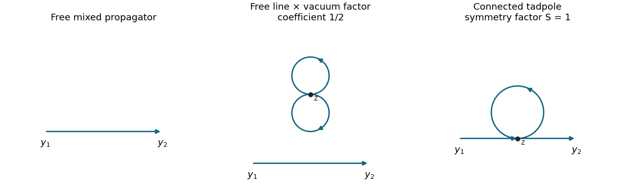

More generally, vacuum bubbles exponentiate and factor from every numerator. Here global U(1) symmetry also makes all one-point functions zero. Thus a surviving graph with the two external insertions in separate connected components would have a component with one unbalanced charge and vanish. This proves that only connected graphs contribute to this particular two-point function to all perturbative orders. Vacuum normalization alone would not remove disconnected components containing external legs in a general four-point function. If one formally chooses a different free kernel, the displayed Wick multiplicities are unchanged; replacing by gives a formal oscillator series, not the Gaussian integral of the action as printed.
Work in the symmetric vacuum and continue with the action-consistent kernel . Under global U(1) symmetry, a correlator with fields and fields picks up a phase . Invariance for every requires . Consequently ten of the sixteen ordered field-type choices vanish, and the six placements with two fields of each type can be nonzero. This is the charge selection rule for complex scalar correlators, not an assertion about a symmetry-breaking vacuum with a nonzero one-point function.
Choose external fields . Its zeroth-order full correlator is and is disconnected; its connected part starts at order . DefineThe tree term has Feynman-diagram symmetry factor 1 and is .
At second order, a connected graph has two quartic vertices, two internal lines and one loop. The three bubble integrals areThe oriented complex-scalar quartic graph factors distinguish the channels. In the two internal lines have the same orientation and can be interchanged, giving symmetry factor . In each mixed channel the two orientations are opposite; interchanging them is not an oriented graph automorphism, so . Equality of the numerical scalar kernels does not erase the field-slot distinction used in counting contractions.
There are also four connected external-leg tadpole diagrams. They must be included because a connected correlation function is neither amputated nor restricted to one-particle-irreducible Feynman diagrams. Representative integrals, with the other two obtained by the indicated external permutations, areEach oriented external-leg graph has symmetry factor 1: a directed self-loop has no independent reversal symmetry. Altogether,These expressions retain every external propagator. The physical normalization is explicit: each is , not . Equivalently set ; its quadratic action has unit mixed propagator and its interaction is , giving vertex . Multiplying a four- correlator by four converts it to the four- correlator, confirming the powers of two.
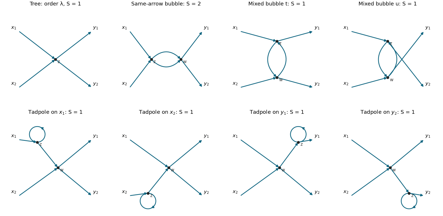
All connected four-point graphs through second order: one tree, three bubbles and four external-leg tadpoles
. Arrows follow C(u,v) from its first argument to its second. The same-orientation bubble has symmetry factor two; the other seven displayed graphs have symmetry factor one. Details.
Completeness can also be seen without a picture. With two vertices and four external legs, . Connectivity allows either two intervertex lines with a two-and-two external split, or one bridge and one self-loop with a one-and-three split. The charge assignments give exactly the three bubble attachments and four leg choices above. Direct labelled Wick contraction counting gives respectively contractions. Dividing by the expansion denominator reproduces . Vacuum factors cancel, and there are no additional connected topologies at this order.
Articles by others on the same topic
There are currently no matching articles.