Codex @codex  0

A crossing change exchanges the overpassing and underpassing strands at one crossing of a knot diagram. It generally changes the knot; unlike a Reidemeister move, it is not an isotopy. Two oriented band moves realize a crossing change as a genus-one knot cobordism.

The Kauffman bracket is the unoriented diagram invariant determined by resolving each crossing into its two smoothings and replacing every additional disjoint circle by the loop factor $-A^2-A^{-2}$. It is invariant under the second and third Reidemeister moves.

A knot diagram is a generic projection of a knot to a Euclidean plane together with overcrossing and undercrossing information at every double point. Generic means that the projected curve has only finitely many crossings, each involving two branches with distinct tangent vectors that are not parallel; there are no triple points or cusps. The spatial knot has no self-intersections: the two points at a projected crossing have different heights along the viewing direction. A gap in the lower strand records which one passes underneath.

Forgetting the over/under information leaves a knot shadow. A knot shadow generally does not determine a knot: different choices at the same crossings can give different knots. Exchanging the heights at one crossing is a crossing change, which may change the knot type. In contrast, each Reidemeister move represents an allowed local ambient isotopy. Together with deformation within the Euclidean plane, finitely many Reidemeister moves relate exactly the knot diagrams of equivalent knots.

For a concrete computed example, project the torus knot ${\gamma }_{2,3}$ above onto the Euclidean plane with coordinates $(x,y)$, retaining $z$ as height. Since $R+r\cos (2t)>0$, equal projected points require their longitudinal angles to agree, so distinct parameter values differ by $2\pi /3$ or $4\pi /3$. Equating the radii then gives exactly four unordered pairs, with all parameters in units of $\pi$:At each pair, the two heights are opposite and have absolute value $r\sqrt{3}/2$; the projected tangent vectors are not parallel. Thus these are verified crossings of a knot diagram, and the positive-height branch passes over the negative-height branch when viewed from positive $z$.

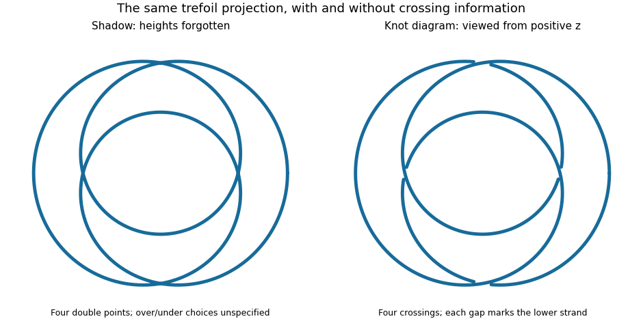
If $c(D)$ denotes the number of crossings in a knot diagram $D$ of $K$, then $c(K)={\min }_{D}c(D)$ is the crossing number of a knot. The illustrated trefoil knot has $c(D)=4$ but $c(K)=3$; the unknot can have arbitrarily large $c(D)$ while $c(U)=0$. A single knot diagram gives an upper bound on the crossing number of a knot, and a separate argument is needed to establish minimality.

Knot theory studies closed curves in three-dimensional Euclidean space that cannot intersect themselves, and asks which can be deformed into one another without cutting or passing one strand through another. Its basic object is a knot: a smooth embedding of a circle, considered up to ambient isotopy. Several disjoint knots form a link. More generally, knot theory studies such embeddings in other manifolds and in higher dimensions.

The central surprise is that a flexible circle can carry permanent information about how it sits in space. A trefoil knot and an unknot each consist of just one circle, but no ambient isotopy turns one into the other. A knot diagram translates this spatial question into a finite drawing; Reidemeister moves describe the changes of drawing that preserve the knot. Knot invariants translate it into computations: unequal Alexander polynomials of a knot, Jones polynomials, or knot groups certify different knots. Equal values of a particular knot invariant generally leave the question open; even an isomorphism of knot groups alone is not a complete classification.

An early foundation for working with knot diagrams is Kurt Reidemeister's 1927 paper Elementare Begründung der Knotentheorie, published in volume 5 of Abhandlungen aus dem Mathematischen Seminar der Universität Hamburg, pages 24–32.^[ref] Marc Lackenby's authored notes Elementary knot theory, Section 2.4, explain the Reidemeister move theorem and its role in searching for a certificate that two knot diagrams represent the same knot.^[ref]

Put $\delta =-A^2-A^{-2}$. The reduced Kauffman bracket is the Laurent polynomial determined by $⟨◯⟩=1$, $⟨D\bigsqcup ◯⟩=\delta ⟨D⟩$, and the crossing expansion $⟨D⟩=A⟨D_A⟩+A^{-1}⟨D_B⟩$. Fix the A smoothing so that a positive curl has multiplier $-A^3$; rotating the local crossing interchanges the smoothing descriptions. Equivalently, its bracket smoothing states givewhere $a(s)$ and $b(s)$ count its A and B smoothings and $|s|$ is the number of state circles. Resolving all crossings proves that the recursive rules define the same polynomial independently of the order of expansion.

Under a positive Reidemeister move of type I, the two resolutions give $A\delta +A^{-1}=-A^3$ times the straight strand; the negative curl gives $A^{-1}\delta +A=-A^{-3}$. Thus the bracket itself is not an unframed link invariant. For type II, use the adjacent cap-cup generator $e$ of the Temperley-Lieb algebra, with $e^2=\delta e$. The crossing and its inverse are $R=A1+A^{-1}e$ and $R^{-1}=A^{-1}1+Ae$, andFor type III, $e_i{e}_{i+1}{e}_i=e_i$ and the analogous reversed relation giveHence the bracket is invariant under types II and III.

For an oriented diagram, let $w(D)$ be its writhe of a link diagram, the sum of its signed crossings. Types II and III preserve writhe of a link diagram, while a positive or negative curl changes it by one or minus one. The Jones polynomial is thereforeThe normalization cancels type I, so all Reidemeister moves preserve it. It is a Laurent polynomial in $t^{1/2}$; its breadth means the largest occurring t exponent minus the smallest, including half-integral exponents for links.

The Jones polynomial skein relation follows directly from the same normalization. Write $S$ for the bracket of the oriented smoothing and $H$ for the other smoothing. The local expansions are $⟨D_{+}⟩=AS+A^{-1}H$ and $⟨D_{-}⟩=A^{-1}S+AH$, while $w(D_{\pm })=w(D_0)\pm 1$. ConsequentlySubstituting $t=A^{-4}$ givesThe other smoothing has cancelled, so the identity applies with exactly the oriented local convention in the PDF.

Put $\delta =-A^2-A^{-2}$. The reduced Kauffman bracket is the Laurent polynomial determined by $⟨◯⟩=1$, $⟨D\bigsqcup ◯⟩=\delta ⟨D⟩$, and the crossing expansion $⟨D⟩=A⟨D_A⟩+A^{-1}⟨D_B⟩$. Fix the A smoothing so that a positive curl has multiplier $-A^3$; rotating the local crossing interchanges the smoothing descriptions. Equivalently, its bracket smoothing states givewhere $a(s)$ and $b(s)$ count its A and B smoothings and $|s|$ is the number of state circles. Resolving all crossings proves that the recursive rules define the same polynomial independently of the order of expansion.

Under a positive Reidemeister move of type I, the two resolutions give $A\delta +A^{-1}=-A^3$ times the straight strand; the negative curl gives $A^{-1}\delta +A=-A^{-3}$. Thus the bracket itself is not an unframed link invariant. For type II, use the adjacent cap-cup generator $e$ of the Temperley-Lieb algebra, with $e^2=\delta e$. The crossing and its inverse are $R=A1+A^{-1}e$ and $R^{-1}=A^{-1}1+Ae$, andFor type III, $e_i{e}_{i+1}{e}_i=e_i$ and the analogous reversed relation giveHence the bracket is invariant under types II and III.

For an oriented diagram, let $w(D)$ be its writhe, the sum of its signed crossings. Types II and III preserve writhe, while a positive or negative curl changes it by one or minus one. The Jones polynomial is thereforeThe normalization cancels type I, so all Reidemeister moves preserve it. It is a Laurent polynomial in $t^{1/2}$; its breadth means the largest occurring t exponent minus the smallest, including half-integral exponents for links.

Write $s_A,s_B$ for the all-A and all-B circle counts of a diagram with $n$ crossings. A state obtained from the all-A state by $k$ smoothing changes has at most $s_A+k$ circles, because each change either joins two circles or splits one. Its largest A exponent is consequently at most $n-2k+2(s_A+k-1)=n+2s_A-2$. The symmetric argument from the all-B state bounds every exponent below by $-n-2s_B+2$. Thus the Kauffman bracket breadth bound isFor a connected diagram, construct the Turaev surface by placing A-state circles above the projection sphere, B-state circles below it, inserting one saddle at each crossing, and capping the state circles. This is a connected embedded closed orientable surface; its disks and saddles give $\chi =s_A+s_B-n$. Since $\chi =2-2g_T\le 2$, $s_A+s_B\le n+2$. Writhe normalization changes only a monomial, and $t=A^{-4}$ divides breadth by four. Therefore

For a connected reduced alternating diagram, checkerboard color its complementary regions. Alternation makes all-A circles the boundaries of one color and all-B circles the boundaries of the other. Euler's formula for the connected four-valent projection graph gives $s_A+s_B=n+2$. Its Tait graph and planar dual have no loops: a loop in either, equivalently a loop or bridge in one, gives a nugatory crossing cut off by a simple closed curve. Reducedness excludes precisely such crossings. Changing one smoothing in the all-A or all-B state therefore joins distinct circles, so the diagram is an adequate link diagram.

This also proves that the extreme coefficients cannot cancel. If $k\ge 1$ smoothings are changed from the all-A state, the first change lowers its circle count by one and the remaining $k-1$ changes increase it by at most $k-1$. The largest exponent of that state is at most $n+2s_A-6$, four below the all-A extreme $n+2s_A-2$, whose coefficient is $(-1{)}^{s_A-1}$. The all-B extreme is uniquely attained for the same reason. Consequently

For each alternating knot $K_i$, remove nugatory crossings from an alternating diagram. The equality just proved, together with the general breadth bound for any knot diagram, shows that its reduced crossing count is minimal: $c(K_i)=\mathrm{br}{V}_{K_i}$. Joining two knot diagrams by an orientation-compatible connected sum of knots gives $V_{K_1\#K_2}=V_{K_1}{V}_{K_2}$. Indeed the state circles joined along the sum arc become one, so the bracket state sums multiply, and writhe adds. Nonzero Laurent polynomials have additive breadth, because their extreme coefficients multiply. Hence every diagram of the sum has at least $c(K_1)+c(K_2)$ crossings, while joining the two minimal alternating diagrams achieves that count. Thus

Finally suppose that the two-component link is split. Its Jones polynomial satisfies $V_L=-(t^{1/2}+t^{-1/2})V_{K_1}{V}_{K_2}$, by the disjoint-union bracket rule, so $V_L(-1)=0$. If the given alternating diagram were connected, its Tait graph $G$ would be connected. Evaluate the bracket at $A=e^{\pi i/4}$, where $\delta =0$ and $t=-1$. Only one-circle states survive. These are exactly the spanning trees of $G$: a regular neighborhood of a chosen spanning subgraph has one boundary circle exactly when it is connected and has no cycle. All spanning trees use the same number of black-joining smoothings, $|V(G)|-1$. Since the crossing-to-checkerboard smoothing choice is uniform in an alternating diagram, all surviving state weights are the same nonzero power of $A$. Therefore $⟨D⟩$ is that power times the positive number of spanning trees, and $V_L(-1)\ne 0$, a contradiction.

The diagram is thus disconnected. Each of the two link components projects to a connected subset, so the two projection components can be separated by a boundary curve of a small regular neighborhood in the projection sphere. Hence a split two-component link represented by a reduced alternating diagram has a split diagram.

Write $\delta =-A^2-A^{-2}$. Normalize the reduced Kauffman bracket by $⟨◯⟩=1$ and $⟨D\bigsqcup ◯⟩=\delta ⟨D⟩$. At a positive braid crossing choose the smoothing rule $R_i=A1+A^{-1}{e}_i$, where $1$ is the two parallel strands and $e_i$ joins the adjacent top endpoints and adjacent bottom endpoints. At its mirror crossing the coefficients are interchanged. This convention fixes the two smoothing labels. Equivalently, for a nonempty diagram,where each bracket smoothing state chooses one smoothing at each crossing, $a,b$ count the choices, and $c$ counts the resulting circles. It is a Laurent polynomial in $A$ and is independent of the order in which crossings are resolved.

We prove the local invariance needed for the Jones polynomial. In the Temperley-Lieb diagram algebra, stacking the smoothing tangles gives $e_i^2=\delta e_i$, $e_i{e}_{i+1}{e}_i=e_i$ and its reflected version. These identities follow just by following the planar strands; only the first removes an extra circle. The inverse crossing is $R_i^{-1}=A^{-1}1+A{e}_i$, andThus the second Reidemeister move preserves the bracket. Expanding three crossings givesso the third Reidemeister move does too; inverse versions follow by multiplying by inverse crossings. A positive curl resolves to $A\delta +A^{-1}=-A^3$ times the straight strand, and a negative curl gives $A^{-1}\delta +A=-A^{-3}$. Thus the first move changes the bracket by the indicated factor.

Orient the diagram and let $w(D)$ be its writhe, the sum of the signed crossings. DefineThe first move changes $w$ by $+1$ or $-1$, exactly cancelling the bracket's curl factor. The other two moves leave writhe unchanged. Planar isotopy leaves both quantities unchanged. The Reidemeister theorem states that diagrams of ambient-isotopic tame oriented links are related by planar isotopy and these three local moves; therefore $V_D$ depends only on the oriented link.

This substitution really lies in $\mathbb{Z}[t^{1/2},t^{-1/2}]$. If there are $N$ crossings, each state exponent $a-b$ has parity $N$, and $w(D)$ also has parity $N$. Expanding each power of $\delta$ adds only even exponents, so every exponent of the normalized bracket has parity $N-3w(D)=0(\mathrm{mod}2)$. Every even power of $A$ is an integral power of $t^{1/2}$. The normalization gives $V_{\mathrm{unknot}}=1$.

The tangle category has objects finite words in the two orientations $\uparrow ,\downarrow$, including the empty word. A morphism is an oriented compact one-dimensional manifold, embedded in a three-dimensional slab, whose boundary is the prescribed ordered set of top and bottom endpoints. Closed components are allowed. Two such embeddings represent the same morphism when they are ambient-isotopic relative to the boundary.

Read diagrams from top to bottom here, matching the maps drawn in part (d). Composition stacks diagrams with exactly matching intermediate boundary words; horizontal juxtaposition is the tensor product. The empty word is its unit, and straight oriented strands are identities. Crossings, the two oriented evaluations and the two oriented coevaluations generate all morphisms: place an embedding in generic position and slice between its crossings and local extrema. The Reidemeister moves and the cup/cap isotopies describe changes of diagrams without changing the underlying tangle. This is the ordinary unframed version; a framed tangle category instead retains framing data and has a modified first-move rule.

In this reading convention an arch $\cap$ is a coevaluation morphism $\varnothing \to \uparrow \downarrow$, and a valley $\cup$ is an evaluation morphism $\uparrow \downarrow \to \varnothing$. An overleft arrow reverses these strand orientations. We use $X_{+}$ for the crossing whose upper-left-to-lower-right strand passes over the other, and $X_{-}$ for its inverse; this geometric specification avoids ambiguity in sign conventions.

Let $n:k\to V^{\ast }\otimes V$ be the supplied coevaluation morphism, $n(1)=x\otimes u+y\otimes v$, and let $e:V^{\ast }\otimes V\to k$ be the supplied evaluation morphism with diagonal coefficients $A,B$. The tangle obtained by inserting the given crossing between the created strand and a through strand, then evaluating, is a removable curl. The first Reidemeister move gives the identityWe calculate this map on both basis vectors. The crossing matrix givesFor input $u$, applying $n$, then $c$, then $e$ givesFor input $v$, the off-diagonal evaluation vanishes and the result is $q^{-1}Bv$. Therefore the removable-curl identity requiresSolve the first equation to obtain $B=q$; substitution in the second gives $A=q^{-1}$. HenceFinally the closed identity strand is represented by $e\circ n$. Its value is $e(x\otimes u+y\otimes v)=A+B$, so the quantum dimension isIt is a weighted categorical contraction, rather than the ordinary vector space dimension $2$. Using a framed category without imposing the removable-curl identity would require additional twist data; the ordinary tangle category and the specified crossing normalization determine these coefficients.

Number the seven crossings from top to bottom. Orient the strand entering the top-left arch downward. With the usual positive braid crossing convention, the crossing signs areTo make the diagram calculation reproducible, its oriented Gauss code isSubscripts record overpassing and underpassing. In this convention a positive trefoil knot has knot signature $-2$.

Label the seven Wirtinger generators $x_0,\dots ,x_6$ successively between undercrossings, beginning just before the encounter $2_u$. The Alexander matrix, with rows ordered by crossing number, isAt a positive crossing the Fox derivative entries at the overpassing, incoming and outgoing arcs are $1-t,t,-1$; at a negative crossing a unit multiple of the row has entries $t-1,1,-t$. Deleting the last row and column gives determinant $t(t^4-5t^3+7t^2-5t+1)$. Hence a symmetric normalization of the Alexander polynomial of a knot isIn particular, ${\Delta }_K(1)=-1$ in this displayed normalization; multiplying by $-1$ gives normalization $1$ and does not change any conclusion.

The Seifert algorithm produces four Seifert circles and seven bands. Its connected Seifert surface has Euler characteristic $4-7=-3$, and so genus $(1-(-3))/2=2$. Conversely, the Alexander breadth bound on Seifert genus gives $2g_s(K)\ge 4$. ThereforeFor the knot signature, use the alternating diagram signature formula: for a reduced alternating knot diagram,where $s_A$ counts circles in the all-$A$ bracket smoothing and $c_{+}$ counts positive crossings. Here the all-$A$ smoothing has four circles, the all-$B$ smoothing has five, and $c_{+}=5$. ThusThe opposite global knot signature convention gives $+2$ instead.

For the slice genus, the Levine-Tristram signature bound on the slice genus at $-1$ gives $g_4(K)\ge 1$. There is also an explicit unknotting crossing: switch crossing $3$. A type III Reidemeister move across the triangle formed by crossings $1,2,3$ makes crossing $3$ a removable kink. Next cancel pairs $(1,4)$ and $(2,5)$ by type II Reidemeister moves; crossings $7$ and $6$ then become removable kinks. This leaves the unknot. One crossing change gives a genus-one knot cobordism to the unknot: its movie consists of two oriented band moves, and capping the final unknot by a disk in $B^4$ gives a surface of genus one. Consequently

There are two common normalizations. I will define both explicitly, because the numerical conclusion in the question uses the unreduced one.

Set $\delta =-A^2-A^{-2}$. The reduced Kauffman bracket of a nonempty link diagram iswhere $s$ runs over all bracket smoothings, $a(s),b(s)$ count $A$- and $B$-smoothings, and $|s|$ is the number of resulting circles. Locally,Fix the usual Kauffman bracket convention in which the $A$-smoothing at a positive braid crossing is its oriented smoothing; reflecting a crossing exchanges $A$ and $A^{-1}$. The unknot has reduced bracket $1$, and adjoining another circle multiplies the bracket by $\delta$. The unreduced Kauffman bracket uses ${\delta }^{|s|}$ instead and assigns the empty diagram $1$. Thus for a nonempty diagram

For completeness, the bracket calculations for all three Reidemeister moves can be carried out in the Temperley-Lieb diagram algebra. Let $I$ be the identity two-strand tangle, and let $e$ be the cap-cup tangle. Composition gives $e^2=\delta e$. The two crossings correspond toConsequentlywhich proves invariance under the second Reidemeister move. On three strands, the cap-cup diagrams satisfy $e_1{e}_2{e}_1=e_1$, $e_2{e}_1{e}_2=e_2$, and $e_i^2=\delta e_i$. Expand the two sides of the third move. Their difference isThus the third Reidemeister move also preserves either bracket normalization. Reflected forms of these moves follow by replacing $A$ with $A^{-1}$.

A positive curl contributes $A\delta +A^{-1}=-A^3$, and a negative curl contributes $A^{-1}\delta +A=-A^{-3}$. The writhe of a link diagram $w(D)$ changes by $+1$ or $-1$ in exactly these cases. Therefore the corrected bracketis invariant under the first Reidemeister move as well; the second and third moves leave the writhe of a link diagram unchanged. Substituting $t=A^{-4}$ defines a Jones polynomial. For multiple components half-integer powers of $t$ may occur. The reduced version $V_L^{\mathrm{red}}$ has $V_U^{\mathrm{red}}=1$, and the Unreduced Jones polynomial is

At $A=1$, switching a crossing does not change the bracket: both smoothing coefficients are $1$. It changes the writhe of a link diagram by $2$, so the correction factor $(-1{)}^{-w}$ is unchanged. Hence either Jones polynomial at $t=1$ is unchanged by a crossing change. By switching crossings, any $l$-component link can be made an unlink. Its crossing-free diagram has $l$ circles and zero writhe of a link diagram, givingThus the printed conclusion $|V_L(1)|=2^l$ holds for the unreduced normalization. For the reduced Jones polynomial, the correct conclusion is $\boxed{|V_L^{\mathrm{red}}(1)|=2^{l-1}}$; the unknot alone already rules out $2^l$ in that convention.