The ruby pressure scale converts a shift of a ruby fluorescence spectral line into pressure. Excitation light produces a fluorescence emission spectrum; fitting its line gives a wavelength . The reference must be measured or assigned at specified reference pressure and temperature. The difference is an observable; interpreting it as pressure requires a pressure calibration and suitable stress conditions.
The original 1972 report found sharp emission shifting toward lower photon energy as pressure increased; it tentatively associated broadening with nonhydrostatic conditions.[ref]
Pressure Measurement Made by the Utilization of Ruby Sharp-Line Luminescence by Richard A. Forman and others. Abstract: direction of R-line shifts and tentative nonhydrostatic interpretation
In use, excitation rejection, a calibrated wavelength axis and a fitted background matter because leakage or background can move an apparent peak. A brighter trace improves counting statistics but does not alone establish a correct pressure scale.The ruby R-line shift compares the same emission feature under two conditions. It is distinct from the Stokes shift, which compares absorption and emission features. In ruby, chromium ions in the corundum crystal provide the electronic transitions; compression changes their local environment and transition energies.[ref]
Stress Measurements in Alumina by Optical Fluorescence: Revisited by Robert F. Cook and Chris A. Michaels. Introduction and hydrostatic-pressure discussion: chromium fluorescence in alumina and stress-sensitive R lines
For consistently defined vacuum wavelengths, the reciprocal relation givesThus a positive wavelength shift means a negative reciprocal shift, and gives lower photon energy; is the Planck constant and the speed of light. For spectroscopic wavenumber, use vacuum wavelength and keep that convention consistent. A calibration specified in air wavelength must retain its convention or be converted consistently. The reciprocal relation is nonlinear: a line exactly linear in is not exactly linear in .
For a purely mathematical check with chosen vacuum wavelengths and , the reciprocal shift is . The small-shift approximation gives , about too large in magnitude. These chosen values illustrate the conversion; they are not measured ruby lines or an additional pressure calibration.
The 1975 experiment mixed powdered sodium chloride and 0.5%-chromium ruby in a 4:1 volume ratio. An Inconel gasket, initially thick with a hole, held the powder and 4:1 methanol–ethanol. At , X-ray diffraction rings on film away gave salt compression; a reference equation of state assigned pressure. After decreasing load, they waited at least five hours and bracketed diffraction exposures with readings to check drift.[ref]
Calibration of the pressure dependence of the R1 ruby fluorescence line to 195 kbar by Gasper J. Piermarini and others. pp. 2774–2775, Experimental Procedures
The recommended linear slope was , with a fit confidence interval of , to . Reference-scale systematic measurement uncertainty remained separate. Above about the medium was only quasihydrostatic; separate range fits checked consistency.[ref]
Calibration of the pressure dependence of the R1 ruby fluorescence line to 195 kbar by Gasper J. Piermarini and others. pp. 2775–2776, Table I and recommended calibration; p. 2778, pressure-distribution discussion
The logical chain is compression to reference pressure, paired with optical shift, then a fitted response. X-ray diffraction supplies the reference comparison during calibration; subsequent ruby readings transfer that scale to other samples. The reference equation of state is therefore part of the meaning of the reported pressure. Changing it can move all calibrated readings together, even if the optical measurements repeat perfectly. A regression residual tests agreement with the chosen reference within the sampled conditions; it cannot independently certify that reference.
Construct a synthetic local calibration to show the calculation independently of the historical data. Choose reference pairs , with shifts in and pressures in . The reference zero is already subtracted. Treat the shifts as exact for this fit and give the three reference pressures equal weights. Minimizing the ordinary least squares objectiveand setting its derivative to zero givesThe regression residuals are . Their weighted moment vanishes, as required by the least-squares normal equations. An unknown reference offset requires fitting an intercept instead; forcing it to zero can bias the slope. If shift errors matter, this elementary fit is insufficient.
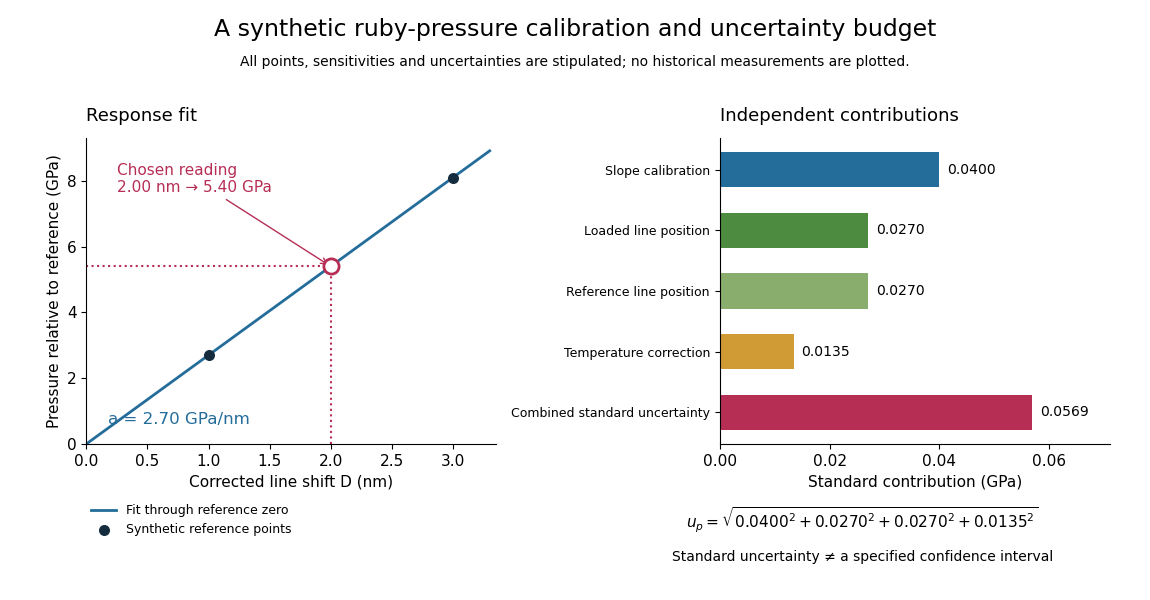
Synthetic ruby pressure scale: fitting the response and propagating measurement uncertainty
. Original stipulated reference points and calculations, not measured historical calibration. The left panel shows the fitted slope and a chosen reading. The right panel separates independent contributions to standard uncertainty; bar lengths are standard contributions, which combine by sums of squares. The assigned slope standard uncertainty includes a hypothetical reference-scale contribution and is not estimated from the three residuals. Details.Use the local measurement modelHere denotes pressure relative to the reference, is calibrated sensitivity, and is a local wavelength sensitivity to temperature at fixed pressure. Choose , and a reading at . The inferred pressure is . These coefficients and readings are stipulated, not measured ruby constants. With the same pressure, a increase in temperature would add to the shift in this model; neglecting it would overestimate pressure by .
Assign independent standard uncertainties , and for the temperature difference. Here is an independently assigned calibration uncertainty, not an estimate from the regression residuals above; treat as exact in this example. First-order propagation of uncertainty follows by differentiating the measurement model:The four standard contributions are , giving . This is a standard uncertainty, not automatically a interval. Correlated reference and loaded wavelength readings require the corresponding covariance term; common wavelength-axis drift may cancel in their difference. Uncertain , nonzero , model inadequacy and unresolved deviatoric stress require a broader budget. Taking more optical readings reduces some random errors while leaving a common reference-scale error.
A single optical shift represents pressure only to the extent that the calibration's mechanical and thermal conditions apply. Under hydrostatic stress, all directions have the same compressive normal stress. Under deviatoric stress, differently oriented ruby grains can respond differently; spatially varying pressure can also superpose shifted lines. These mechanisms can produce different optical signals at equal mean pressure.[ref]
Stress Measurements in Alumina by Optical Fluorescence: Revisited by Robert F. Cook and Chris A. Michaels. Sections 1–2: stress-sensitive fluorescence shifts and crystallographic stress components
The 2001 account describes scanning local line positions and measuring line width over an extended region. The former resolves spatial differences; the latter supplies a rapid warning.[ref]
High Pressure X-Ray Crystallography With the Diamond Cell at NIST⁄NBS by Gasper J. Piermarini. Section 4.2, Methods I and II
Neither a broadened line nor a narrow one uniquely determines the stress tensor. Instrument resolution, temperature variation and unresolved overlapping signals can also affect width. A small observed region can have a narrow line while differing from another region. Compare locations, reference traces and instrument settings before treating width as evidence for a particular mechanical explanation. These are proposed diagnostic checks, not additional historical controls attributed to the 1975 experiment.
Temperature is another independent input. A useful local expansion is : one measured shift cannot determine both unknowns. Measure or control temperature, or supply a second independently calibrated observable. The coefficients need not remain constant across a large range. Even when a pressure sensitivity transfers over some temperatures, the reference line, line width and practical readout quality can change.
The historical high-temperature account reports degrading pressure measurement quality above about .[ref]
High Pressure X-Ray Crystallography With the Diamond Cell at NIST⁄NBS by Gasper J. Piermarini. Section 4.1, high-temperature cell and readout-quality discussion

