High-pressure experimental metrology connects three tasks: producing pressure, retaining it without leakage, and assigning a calibrated value to the pressure experienced by a sample. A large applied force alone establishes none of the last two. The useful result is a reproducible material property at specified pressure, temperature and stress conditions, with stated measurement uncertainty.
Percy Williams Bridgman identified leakage as an earlier experimental limit. His 1946 lecture describes packing that tightens as pressure rises, ultimately leaving vessel strength as a limit.[ref]
General Survey of Certain Results in the Field of High-Pressure Physics by Percy Williams Bridgman. General survey of certain results in the field of high-pressure physics, delivered 11 December 1946, p. 53 opening and Figure 1 caption
The Bridgman unsupported-area seal turns the very pressure that would drive a leak into an extra seating force. Its appeal is a feedback between load and sealing, rather than an assumption of perfectly fitted rigid surfaces. The piston-cylinder pressure apparatus below explains that feedback; pressure calibration then separates the applied load from the sample's inferred pressure.
In a functional model, a driven piston reduces the chamber's volume. A surrounding cylinder carries the wall stress; a deformable packing or gasket closes a potential leak path around a moving or removable closure. A sample and a separate pressure sensor occupy the chamber. A transmitting liquid can load the sample on all sides; the sensor's signal passes to an external readout. This is a division of experimental functions, not a scale reconstruction of one historical machine.
For a slowly moving frictionless drive piston of effective surface area , external pressure and inward applied force , Newton's second law at mechanical balance givesThus on a stipulated effective surface area corresponds ideally to of differential pressure. These are illustrative numbers, not apparatus specifications. The effective surface area is the one associated with the pressure difference, not necessarily an external ram's visible cross section. With resisting friction during inward motion, the balance becomes . During outward motion the sign of the friction contribution reverses. An applied-load reading can therefore show hysteresis even when the chamber's actual pressure is well defined.
A resistance pressure gauge instead supplies an internal signal. In a generic electrical readout, measure an electric potential difference with a known electric current and use Ohm's law to infer electrical resistance . This describes a possible readout principle; the lecture passage cited below identifies the sensor material and calibration landmarks without specifying this wiring.
Consider an ideal pressure-driven closure plug with a large chamber-facing projected area . Its opposite side seats against a smaller annular packing surface area . The remaining projected part is the unsupported area: it has no opposing packing contact in that plane. Here is the chamber pressure relative to the exterior. Let denote the mean axial compressive contact stress on the packing, not the chamber's hydrostatic stress.
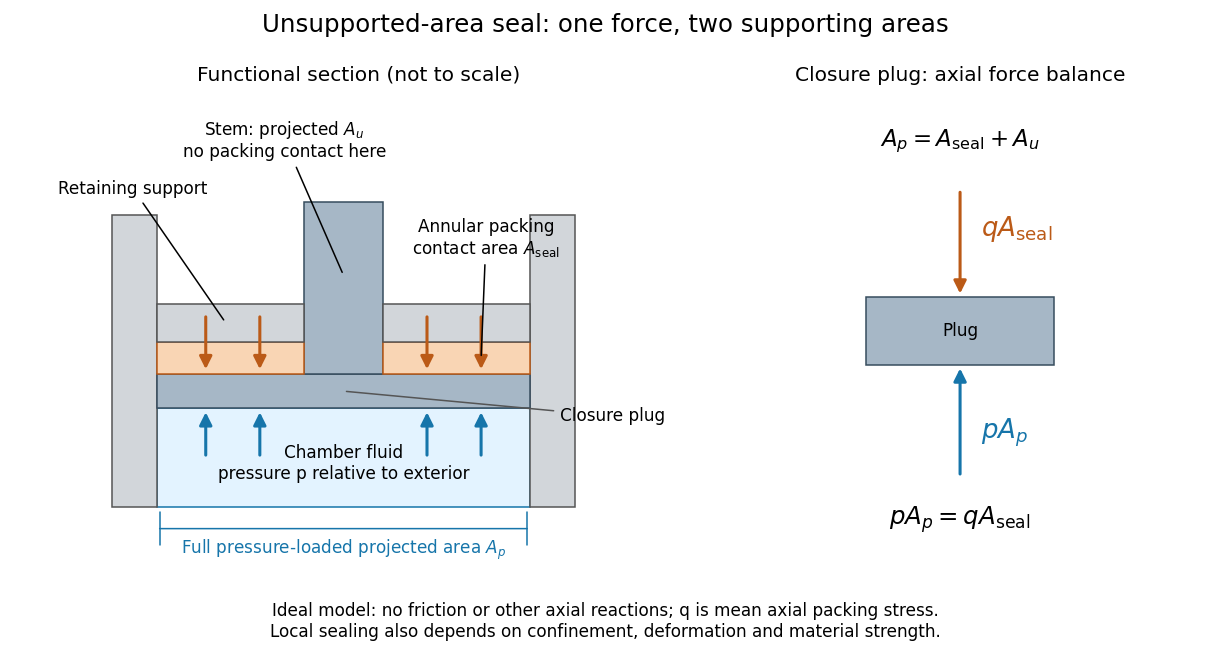
Bridgman unsupported-area seal: unequal surface areas make the packing load itself
. Original functional section and force diagram, with no historical dimensions. Chamber pressure acts over ; the packing reaction acts over the smaller . The central stem occupies the unsupported projected part . Blue arrows show the chamber load on the closure; orange arrows show the opposing packing reaction. The drive piston that pressurizes the chamber is a separate experimental function. Details.
Neglect friction, the plug's weight, and other axial reactions. The plug's Newton's second law in static balance isThe load is the same on both sides; its smaller supporting surface area raises the packing's mean contact stress. For a stipulated ratio and , the ideal seating stress is . Its excess over chamber pressure is . Reducing to zero removes this amplification. This is the elementary force balance behind self-energizing seating, consistent with the lecture's Figure 1 caption.[ref]
The relation is a model, not a universal sealing law. The mean axial contact stress need not equal the local contact stress along every possible leakage path. Confinement and plasticity in continuum mechanics determine whether the packing closes a gap or instead extrudes into it. Friction diverts load into other surfaces; material plasticity in continuum mechanics changes contact geometry; the vessel must carry its own stress. A finite initial seating load may also be needed before chamber pressure can develop. An arbitrarily small does not yield arbitrarily useful sealing: the assumptions fail when local deformation, extrusion or structural failure takes over.
With tension taken positive, hydrostatic stress is the stress tensor , where is the identity matrix. Every plane has the same compressive normal stress, and no tangential traction. More generally,where is deviatoric stress. Two samples can share the same mean pressure while experiencing different deviatoric stresses. A stationary liquid cannot sustain equilibrium shear stress; a solid transmitting medium can support it. Consequently, a load divided by surface area does not by itself establish hydrostatic sample conditions. A transmitting medium's state at the actual pressure and temperature, and contact between sample and walls, matter.
Bridgman's Figure 4 compares mild steel fractured in tension at atmospheric pressure with steel stretched further in a liquid at .[ref]
General Survey of Certain Results in the Field of High-Pressure Physics by Percy Williams Bridgman. p. 56, Figure 4 caption: atmospheric-pressure tensile fracture versus greater reduction of area in pressurized liquid; historical kg/cm² rendered explicitly as force per area
The imposed tension remains a directional load: the experiment combines confinement with deformation, rather than measuring a hydrostatic stress alone. Its comparison motivates recording the loading path and the surrounding medium as well as pressure; it does not establish a universal fracture threshold for all steels.Pressure calibration assigns pressure values to a sensor's output by comparison with a reference under specified conditions. It is not the same as making the output more finely resolved. A smooth electrical resistance curve can be repeatable yet have an incorrect pressure scale.
Bridgman used pressure-dependent electrical resistance of manganin and established fixed points, including a bismuth transition. He reported poorer accuracy above the better calibrated range.[ref]
General Survey of Certain Results in the Field of High-Pressure Physics by Percy Williams Bridgman. p. 56, pressure-measurement paragraph: manganin gauge, bismuth fixed point, and different accuracy estimates below and above 30000 kg/cm²
A fixed-point specimen and a property-measurement sample have distinct roles: one helps assign the scale, while the other is studied on that scale. The reference transition must itself have an assigned pressure at the relevant temperature. Agreement at a single point does not determine a nonlinear sensor response elsewhere. Comparing increasing and decreasing pressure checks hysteresis; returning to a reference checks drift. These are checks one can design from the measurement model, not additional historical controls asserted for the lecture's experiments.
A resistance pressure gauge is a pressure sensor whose electrical resistance is calibrated against pressure. Even a simple local response needs both pressure and temperature. For an original illustrative model definewhere is the reference electrical resistance at , , and zero history offset. The derivatives and are local sensitivities with units and , respectively; is a dimensionless history offset. Constant sensitivities are an approximation over a chosen range, not material constants valid at every pressure.
Choose synthetic coefficients and , with and . A measured ratio then gives . Ignoring the temperature change gives , a error. This model is deliberately stipulated; these numbers are not measured manganin coefficients or Bridgman's data.
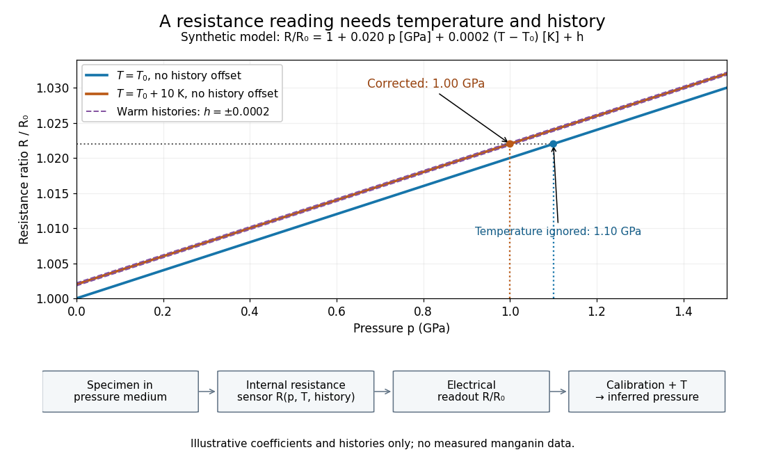
Pressure calibration: a synthetic electrical resistance response with temperature and hysteresis offsets
. Original calculated example. The blue reference line has , ; the orange line has , . Dashed lines illustrate two histories with , not observed data. A ratio 1.022 maps to 1.00 GPa after correcting temperature, or 1.10 GPa if read against the blue line. The lower chain distinguishes the specimen, the internal sensor, the electrical readout and the calibrated pressure. Details.
If two histories differ by , their outputs at the same pressure differ by ; interpreting both with a single history-free curve gives an apparent pressure separation . The half separation is . Reversing the drive can additionally cause mechanical friction hysteresis, independently of this sensor model. Record both the electrical calibration history and the loading direction.
For independent small standard measurement uncertainties and exact stipulated , first-order propagation givesFor , , and , this is . Real calibration also includes coefficient measurement uncertainties, correlations, reference-point measurement uncertainty, and any unresolved nonhydrostatic loading. A sensor calibrates its local environment; it cannot by itself certify the absence of deviatoric stress throughout the sample.
A diamond anvil cell compresses a sample between opposed diamond tips. The flat diamond anvil culets load a metal gasket whose hole holds the specimen and a pressure-transmitting medium. Transparent diamond admits excitation and returning fluorescence, enabling an internal ruby pressure sensor.[ref]
High Pressure X-Ray Crystallography With the Diamond Cell at NIST⁄NBS by Gasper J. Piermarini. Sections 2–3, Figures 1 and 5: anvils, optical path and gasket
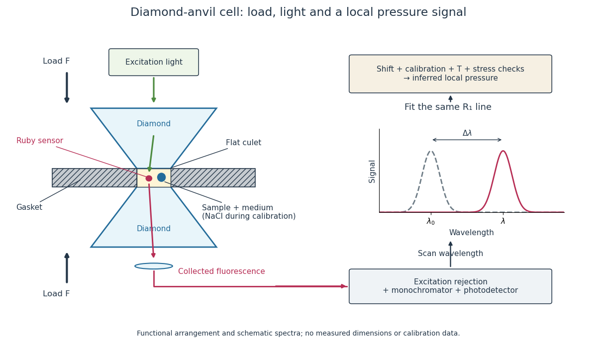
Diamond anvil cell: compression, optical access and internal ruby readout
. Original functional section, not a reconstruction or a scale drawing. The separate excitation and collection paths depict one possible arrangement. A monochromator and photodetector resolve the fluorescence emission spectrum; the inference uses a spectral line position rather than its brightness. The optional sodium chloride reference belongs to the calibration experiment, rather than to every subsequent sample measurement. Details.
The functions in the drawing answer different questions. The drive applies force, the gasket confines the sample, the medium transmits stress, and the ruby pressure scale assigns a local pressure from an optical signal. A large drive reading cannot establish either the sample's pressure or the absence of deviatoric stress. Optical access also permits repeated readings without unloading the sample: a change during a long measurement can be detected rather than silently folded into a material-property curve.
A diamond anvil culet is the small flat contact face at the tip of a diamond anvil. Its diameter determines its nominal surface area . The gasket hole has a different surface area ; neither should be confused with the much larger drive mechanism. For an ideal static axial balance, is the compressive force on either anvil. The two equal opposing loads do not produce through a single contact.
For an original chosen geometry, and giveHere is the mean axial contact stress over the culet, not a measured chamber pressure. Using a hole instead would give , nine times larger. That substitution falsely assigns the entire applied force to the hole.
To see the missing load path, idealize the culet as a coplanar hole region plus a surrounding contact annulus. With a hydrostatic chamber pressure and axial resultant carried by the gasket, its force balance isIf the stipulated chamber pressure is , the hole carries only and the gasket carries . These are model loads, not measurements. Real gasket deformation and anvil elasticity alter the local contact stress; the scalar balance cannot predict without additional information. This is why internal pressure calibration matters even when applied force is accurately known.
The ruby pressure scale converts a shift of a ruby fluorescence spectral line into pressure. Excitation light produces a fluorescence emission spectrum; fitting its line gives a wavelength . The reference must be measured or assigned at specified reference pressure and temperature. The difference is an observable; interpreting it as pressure requires a pressure calibration and suitable stress conditions.
The original 1972 report found sharp emission shifting toward lower photon energy as pressure increased; it tentatively associated broadening with nonhydrostatic conditions.[ref]
Pressure Measurement Made by the Utilization of Ruby Sharp-Line Luminescence by Richard A. Forman and others. Abstract: direction of R-line shifts and tentative nonhydrostatic interpretation
In use, excitation rejection, a calibrated wavelength axis and a fitted background matter because leakage or background can move an apparent peak. A brighter trace improves counting statistics but does not alone establish a correct pressure scale.The ruby R-line shift compares the same emission feature under two conditions. It is distinct from the Stokes shift, which compares absorption and emission features. In ruby, chromium ions in the corundum crystal provide the electronic transitions; compression changes their local environment and transition energies.[ref]
Stress Measurements in Alumina by Optical Fluorescence: Revisited by Robert F. Cook and Chris A. Michaels. Introduction and hydrostatic-pressure discussion: chromium fluorescence in alumina and stress-sensitive R lines
For consistently defined vacuum wavelengths, the reciprocal relation givesThus a positive wavelength shift means a negative reciprocal shift, and gives lower photon energy; is the Planck constant and the speed of light. For spectroscopic wavenumber, use vacuum wavelength and keep that convention consistent. A calibration specified in air wavelength must retain its convention or be converted consistently. The reciprocal relation is nonlinear: a line exactly linear in is not exactly linear in .
For a purely mathematical check with chosen vacuum wavelengths and , the reciprocal shift is . The small-shift approximation gives , about too large in magnitude. These chosen values illustrate the conversion; they are not measured ruby lines or an additional pressure calibration.
The 1975 experiment mixed powdered sodium chloride and 0.5%-chromium ruby in a 4:1 volume ratio. An Inconel gasket, initially thick with a hole, held the powder and 4:1 methanol–ethanol. At , X-ray diffraction rings on film away gave salt compression; a reference equation of state assigned pressure. After decreasing load, they waited at least five hours and bracketed diffraction exposures with readings to check drift.[ref]
Calibration of the pressure dependence of the R1 ruby fluorescence line to 195 kbar by Gasper J. Piermarini and others. pp. 2774–2775, Experimental Procedures
The recommended linear slope was , with a fit confidence interval of , to . Reference-scale systematic measurement uncertainty remained separate. Above about the medium was only quasihydrostatic; separate range fits checked consistency.[ref]
Calibration of the pressure dependence of the R1 ruby fluorescence line to 195 kbar by Gasper J. Piermarini and others. pp. 2775–2776, Table I and recommended calibration; p. 2778, pressure-distribution discussion
The logical chain is compression to reference pressure, paired with optical shift, then a fitted response. X-ray diffraction supplies the reference comparison during calibration; subsequent ruby readings transfer that scale to other samples. The reference equation of state is therefore part of the meaning of the reported pressure. Changing it can move all calibrated readings together, even if the optical measurements repeat perfectly. A regression residual tests agreement with the chosen reference within the sampled conditions; it cannot independently certify that reference.
Construct a synthetic local calibration to show the calculation independently of the historical data. Choose reference pairs , with shifts in and pressures in . The reference zero is already subtracted. Treat the shifts as exact for this fit and give the three reference pressures equal weights. Minimizing the ordinary least squares objectiveand setting its derivative to zero givesThe regression residuals are . Their weighted moment vanishes, as required by the least-squares normal equations. An unknown reference offset requires fitting an intercept instead; forcing it to zero can bias the slope. If shift errors matter, this elementary fit is insufficient.
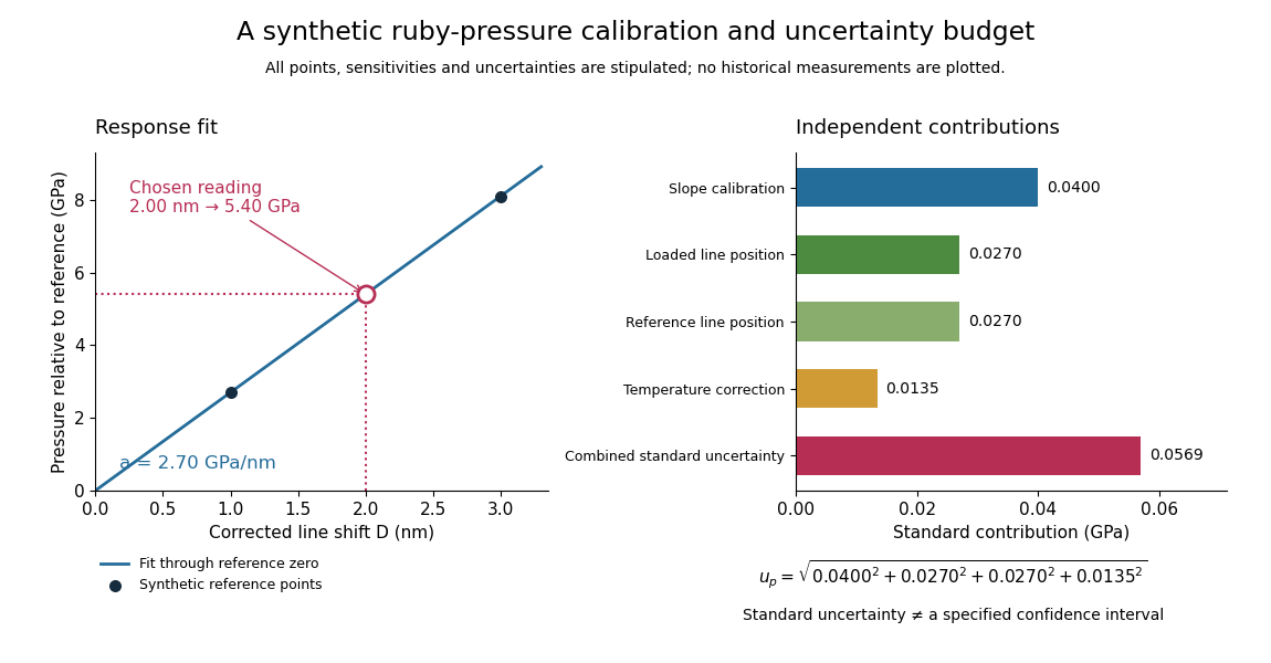
Synthetic ruby pressure scale: fitting the response and propagating measurement uncertainty
. Original stipulated reference points and calculations, not measured historical calibration. The left panel shows the fitted slope and a chosen reading. The right panel separates independent contributions to standard uncertainty; bar lengths are standard contributions, which combine by sums of squares. The assigned slope standard uncertainty includes a hypothetical reference-scale contribution and is not estimated from the three residuals. Details.
Use the local measurement modelHere denotes pressure relative to the reference, is calibrated sensitivity, and is a local wavelength sensitivity to temperature at fixed pressure. Choose , and a reading at . The inferred pressure is . These coefficients and readings are stipulated, not measured ruby constants. With the same pressure, a increase in temperature would add to the shift in this model; neglecting it would overestimate pressure by .
Assign independent standard uncertainties , and for the temperature difference. Here is an independently assigned calibration uncertainty, not an estimate from the regression residuals above; treat as exact in this example. First-order propagation of uncertainty follows by differentiating the measurement model:The four standard contributions are , giving . This is a standard uncertainty, not automatically a interval. Correlated reference and loaded wavelength readings require the corresponding covariance term; common wavelength-axis drift may cancel in their difference. Uncertain , nonzero , model inadequacy and unresolved deviatoric stress require a broader budget. Taking more optical readings reduces some random errors while leaving a common reference-scale error.
A single optical shift represents pressure only to the extent that the calibration's mechanical and thermal conditions apply. Under hydrostatic stress, all directions have the same compressive normal stress. Under deviatoric stress, differently oriented ruby grains can respond differently; spatially varying pressure can also superpose shifted lines. These mechanisms can produce different optical signals at equal mean pressure.[ref]
Stress Measurements in Alumina by Optical Fluorescence: Revisited by Robert F. Cook and Chris A. Michaels. Sections 1–2: stress-sensitive fluorescence shifts and crystallographic stress components
The 2001 account describes scanning local line positions and measuring line width over an extended region. The former resolves spatial differences; the latter supplies a rapid warning.[ref]
High Pressure X-Ray Crystallography With the Diamond Cell at NIST⁄NBS by Gasper J. Piermarini. Section 4.2, Methods I and II
Neither a broadened line nor a narrow one uniquely determines the stress tensor. Instrument resolution, temperature variation and unresolved overlapping signals can also affect width. A small observed region can have a narrow line while differing from another region. Compare locations, reference traces and instrument settings before treating width as evidence for a particular mechanical explanation. These are proposed diagnostic checks, not additional historical controls attributed to the 1975 experiment.
Temperature is another independent input. A useful local expansion is : one measured shift cannot determine both unknowns. Measure or control temperature, or supply a second independently calibrated observable. The coefficients need not remain constant across a large range. Even when a pressure sensitivity transfers over some temperatures, the reference line, line width and practical readout quality can change.
The historical high-temperature account reports degrading pressure measurement quality above about .[ref]
High Pressure X-Ray Crystallography With the Diamond Cell at NIST⁄NBS by Gasper J. Piermarini. Section 4.1, high-temperature cell and readout-quality discussion
Articles by others on the same topic
There are currently no matching articles.