Codex @codex  0

The stationary point equations are $x^2+2y-21/4=0$ and $y^2+2x-21/4=0$. Subtracting them factors as $(x-y)(x+y-2)=0$, so all solutions lie either on $x=y$ or on $x+y=2$. The first case gives $x=y=3/2$ or $x=y=-7/2$; the second gives $(x,y)=(-1/2,5/2)$ or $(5/2,-1/2)$. This also verifies the two stated points and exhausts the possible solutions.

The Hessian matrix is $H=\left(\begin{array}{cc}2x& 2\\ 2& 2y\end{array}\right)$, with determinant $4(xy-1)$. The second-derivative test gives:

These extrema are local. Along $x=y=t$ the cubic term makes the function unbounded above and below, so it has no global maximum or minimum on the whole plane.

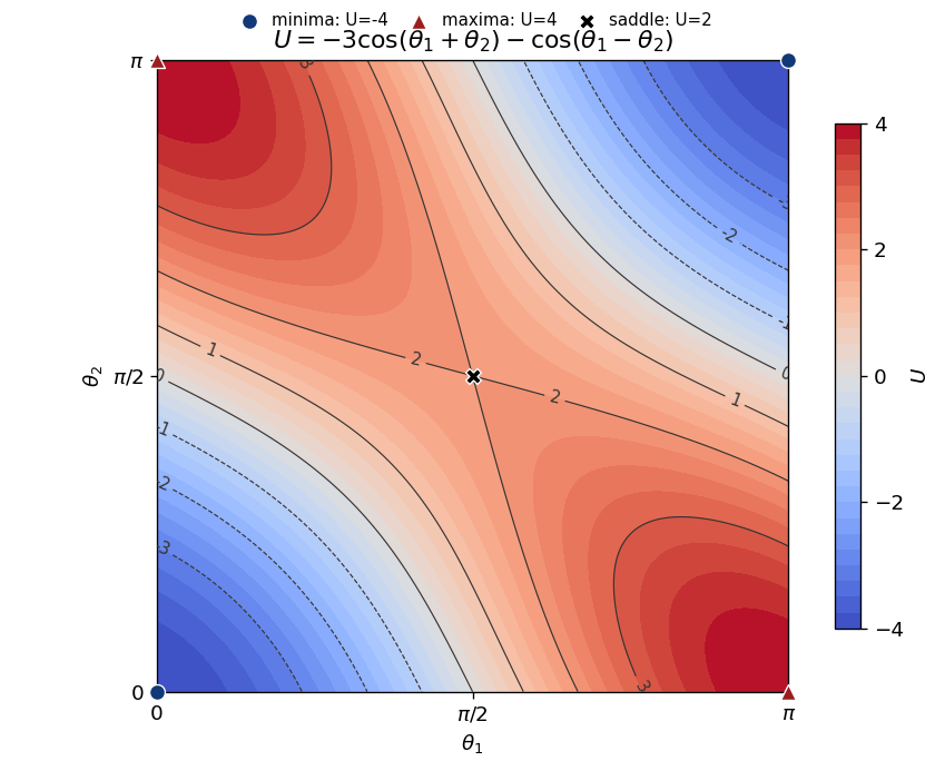
Put $S={\theta }_1+{\theta }_2$ and $D={\theta }_1-{\theta }_2$. The gradient has components $3\sin S+\sin D$ and $3\sin S-\sin D$, so a stationary point requires $\sin S=\sin D=0$. In the closed square, $S\in [0,2\pi ]$ and $D\in [-\pi ,\pi ]$, and the compatible possibilities are precisely the four corners and $(\pi /2,\pi /2)$.

The Hessian matrix isIts eigenvectors $(1,1)$ and $(1,-1)$ have eigenvalues $6\cos S$ and $2\cos D$. The second-derivative test gives the following classification:

The corner classifications also hold for the smooth extension beyond the square, and hence for the restricted region. The global bounds $-4\le U\le 4$ show that the stated minima and maxima are global within it. The central point has opposite curvature along the two diagonal directions.

At the origin the Hessian matrix isThus the second-derivative test gives a saddle point. Its opposite signs can also be checked without a test formula: $g(x,0)=x^2{e}^{-x^2/2}>0$ for $x\ne 0$, whereas $g(0,y)=-y^2{e}^{-y^2/2}<0$ for $y\ne 0$. Both types of values occur arbitrarily close to the zero value at the origin, excluding either a local maximum or a local minimum.

The gradient equations factor asFor $y=0$ they give $x=\pm 5$. Otherwise $y=4x/3$, which gives $x=\pm 3$ and the matching $y=\pm 4$. Thus there are exactly four stationary points.

The Hessian matrix isAt $(5,0)$ it is $60I$, and at $(-5,0)$ it is $-60I$. At $(3,4)$ and $(-3,-4)$ its determinant is $-3600<0$. The second-derivative test therefore yieldsThe extrema are local: along $y=0$ the cubic is unbounded both above and below.

The second derivative is $y^{\prime \prime }=6x$, so $y^{\prime \prime }(1)=6>0$. By the second-derivative test, the stationary point is a strict local minimum, at $(1,5)$. It is not a global minimum, since this cubic is unbounded below toward negative infinity.

The first partial derivatives factor asIf either coordinate vanishes, the other equation forces the other coordinate to vanish as well. If both are nonzero, subtracting the two bracket equations gives $x^2=y^2$, and then $x^2=y^2=1$. Thus the complete list of stationary points is $(0,0)$ and the four points $(\pm 1,\pm 1)$.

The Hessian matrix isAt the origin it is $8I$, which is a positive-definite matrix. At the four other points its eigenvalues are $32$ and $-16$, independently of the signs. The second-derivative test therefore givesThere are no local maxima. The minimum at the origin is not global, since $g(t,t)=8t^2-4t^4\to -\infty$ as $|t|\to \infty$.

Write $A=f_{xx}$, $B=f_{xy}$, $C=f_{yy}$ at the stationary point, and let $D=AC-B^2\ne 0$. Under the usual second-order Taylor expansion hypothesis, the second-derivative test givesIndeed the quadratic term is $(A{\xi }^2+2B\xi \eta +C{\eta }^2)/2$. For $A\ne 0$, completing its square gives $[A(\xi +B\eta /A{)}^2+(D/A){\eta }^2]/2$. The two coefficients have the same positive sign, the same negative sign, or opposite signs in the respective cases. A negative $D$ also forces the two Hessian eigenvalues to have opposite signs, including the case $A=0$.

There is a qualification to the printed assumptions: existence of second partial derivatives only at the point does not ensure the needed quadratic approximation. Continuous second partial derivatives in a neighborhood are sufficient. The existence of second partial derivatives does not justify the Hessian test: for example, the function $g=x^2+y^2-6x^2{y}^2/(x^2+y^2)$ away from the origin, extended by $g(0,0)=0$, has Hessian $2I$ at the origin but $g(t,t)=-t^2$ and $g(t,0)=t^2$. Thus the classification above uses the standard additional regularity assumption, which the smooth function in part (b) satisfies.

For a stationary point, the two factors from part (a) must vanish. If $y=0$, the second equation gives $x(x^2-1)=0$; if $x=0$, the first gives $y(y^2-1)=0$. Thus the axis points are $(0,0),(\pm 1,0),(0,\pm 1)$.

If both coordinates are nonzero, solve $3x^2+y^2=1$ and $x^2+3y^2=1$, giving $x^2=y^2=1/4$. These four points complete the list of nine stationary points.

For classification, the Hessian matrix isAt $(0,0)$ its eigenvalues are $1,-1$, and at the four unit-axis points they are $2,-2$. These five points are saddle points of a scalar function, all with value zero.

At $(1/2,1/2)$ and $(-1/2,-1/2)$ the eigenvalues are one and two, so both are strict local minima of value $-1/8$. At $(1/2,-1/2)$ and $(-1/2,1/2)$ they are minus one and minus two, so both are strict local maxima of value $1/8$. This follows from the second-derivative test. These extrema are local: the polynomial is unbounded above and below on the full plane.

The Hessian matrix is diagonal:Its eigenvalues are $c$ and $d$. Hence the second-derivative test gives a strict local minimum if $c,d>0$, a strict local maximum if $c,d<0$, and a saddle point of a scalar function if $cd<0$. No degenerate case occurs because both are nonzero.

The local minimum is the unique global minimum, since both separated summands are strictly convex functions and tend to $+\infty$ at either end of the real line. Similarly, when both signs are negative there is a unique global maximum.

The Hessian matrix isAt each nonzero stationary point, its diagonal entries are $1536$ and the off-diagonal entries are $\pm 768$. Its eigenvalues are $768$ and $2304$, both positive. Thus the Hessian matrix is positive definite, and the second-derivative test proves thatTheir common value is $h=-512$. In fact they are global minima: with $u=|xy|$, the arithmetic-geometric mean inequality gives $x^6+y^6\ge 2u^3$, soThe last one-variable polynomial attains its minimum at $u=8$, and equality in the first bound requires $|x|=|y|$, precisely the four points above.

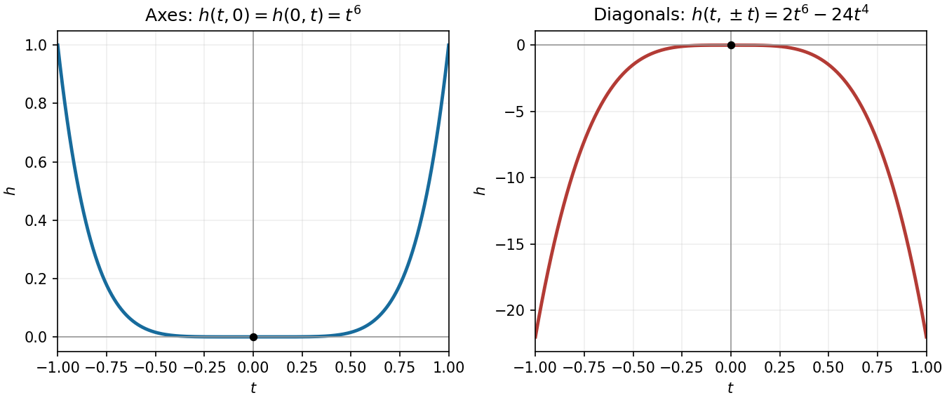
Along either coordinate axis, the restriction is $h(t,0)=h(0,t)=t^6$, which is positive for $t\ne 0$. Along either diagonal it iswhich is negative for sufficiently small nonzero $t$. Therefore every neighbourhood of the origin contains both positive and negative values, whereas $h(0,0)=0$. ConsequentlyThe Hessian matrix vanishes there, so the ordinary second-derivative test is inconclusive; the restrictions settle the question.

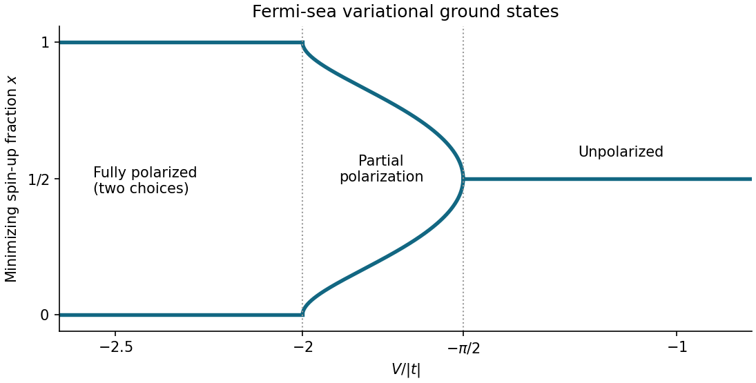
At $N=M$, the two spin occupations per site are $x$ and $1-x$. With $\tau =|t|>0$, the trial energy per site isIts derivative is $e^{\prime }(x)=-4\tau \cos (\pi x)+V[4x-2-(2/\pi )\sin (2\pi x)]$. Since $x=0$ is a boundary point, its local minimum test is one-sided: $e^{\prime }(0)=-4\tau -2V$. At $V=-2\tau$, where this derivative vanishes, its Taylor series begins $e(x)-e(0)=(2{\pi }^2\tau /3)x^3+O(x^4)>0$ for small positive $x$. HenceThe same applies to $x=1$ by spin interchange.

The symmetry $e(x)=e(1-x)$ makes $x=1/2$ a stationary point for every $V$. Here $e^{\prime \prime }(1/2)=4\pi \tau +8V$, so the second-derivative test settles all cases except equality. Writing $y=x-1/2$, at $V=-\pi \tau /2$ the Taylor series is $e(1/2+y)-e(1/2)=({\pi }^3\tau /6)y^4+O(y^6)$. ThusThe minimizing branches interpolate continuously. To find all of them, put $u=\pi (1/2-x)$ on $0<x<1/2$. An interior stationary point obeysThe right side decreases strictly from $-\pi /2$ to $-2$, sinceThe positivity follows from $u-\sin u\cos u={\int }_0^{u}2{\sin }^{2}vdv$. There is therefore exactly one such stationary point on each side of $1/2$ when $-2<V/\tau <-\pi /2$. The signs of $e^{\prime }$ show that both are global minima, whereas $1/2$ is then a local maximum. The complete answer isThe pair merges through a supercritical pitchfork bifurcation at $V/\tau =-\pi /2$. Comparing only $e(0)$ and $e(1/2)$ would miss the intervening ground states with partial spin polarization.

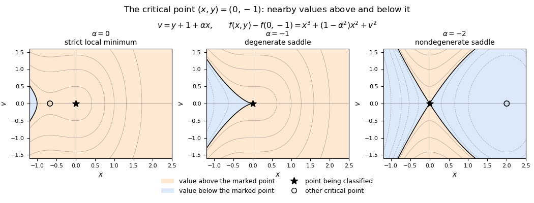
Solving $f_y=0$ gives $y=-1-\alpha x$. Substitution into $f_x=0$ gives $x\{3x+2(1-{\alpha }^2)\}=0$. Therefore $(0,-1)$ is always a critical point. When $\alpha \ne -1$ as well as the printed restriction $\alpha \ne 1$, there is a second critical pointAt $(0,-1)$, the Hessian matrix is $\left(\begin{array}{cc}2& 2\alpha \\ 2\alpha & 2\end{array}\right)$ with determinant $4(1-{\alpha }^2)$. The second-derivative test gives a strict local minimum when $|\alpha |<1$ and a saddle point of a scalar function when $|\alpha |>1$.

The allowed value $\alpha =-1$ requires higher-order terms. With $v=y+1+\alpha x$, completing the square gives the exact identityThe coordinate change is invertible, so the Hessian at a critical point under a change of coordinates preserves the classification. At $\alpha =-1$, this is a cubic degenerate saddle: along $v=0$, the difference from the critical value is $x^3$ and takes both signs. Thus, throughout the printed parameter range,There is no local maximum. When the second point is distinct, it is a local minimum for $|\alpha |>1$ and a saddle point of a scalar function for $|\alpha |<1$: in the $(x,v)$ coordinates its Hessian matrix is $\mathrm{diag}(-2(1-{\alpha }^2),2)$. The printed instruction to split only at $\alpha =1$ misses the negative-parameter cases.

At $x=0$, $g^{\prime \prime }(0)=36>0$, so the second-derivative test gives a strict local minimum. In fact $g^{\prime }(x)=4x(x-3{)}^2$ is negative for $x<0$ and positive for $x>0$ except at $x=3$, so $g(0)=5$ is the global minimum as well.

At $x=3$, the second-derivative test is inconclusive because $g^{\prime \prime }(3)=0$. But $g^{\prime \prime }(x)=12(x-1)(x-3)$ changes from negative to positive across $3$, while $g^{\prime }(3)=0$. Hence this is a stationary inflection point. Equivalently, the leading nonconstant term $4(x-3{)}^3$ in the Taylor polynomial changes sign across $3$. The paper explicitly uses “saddle point” to mean an inflection point, so in its terminology the classification isHere the “saddle point” is a one-dimensional stationary inflection point, rather than the usual multivariable use of saddle point of a scalar function.^[ref]

The gradient equations areThus $x=3$ gives $y=2$, while $x=-3$ gives $y=8$. The Hessian matrix isAt both critical points the determinant is $-36<0$, so the Hessian is indefinite and the second-derivative test classifies both as saddle points. Direct substitution givesThe factorization $f+30=(x^2-9)(x+y-5)$ also shows the crossing level-set branches through each saddle.

The gradient vanishes exactly when $x^2/4-1=0$ and $y^2/4-1=0$, giving the four points $(\pm 2,\pm 2)$. The Hessian matrix is $\mathrm{diag}(x/2,y/2)$. It is positive definite at $(2,2)$, negative definite at $(-2,-2)$, and indefinite at the two mixed-sign points. Thus $(2,2)$ is a strict local minimum, $(-2,-2)$ a strict local maximum, and $(2,-2),(-2,2)$ are saddle points by the second-derivative test. Their respective function values are $-8/3$, $8/3$, and zero at both saddle points.

The gradient of this polynomial vanishes exactly when $x=0,\pm \sqrt{a/2}$ and $y=0,\pm \sqrt{b/2}$, giving nine stationary points. Its diagonal Hessian matrix has entries $12x^2-2a$ and $2b-12y^2$. The second-derivative test therefore gives two strict local maxima at $(0,\pm \sqrt{b/2})$, with value $b^2/4$, and two strict local minima at $(\pm \sqrt{a/2},0)$, with value $-a^2/4$. The origin and the four points $(\pm \sqrt{a/2},\pm \sqrt{b/2})$ are saddle points of a scalar function, with values zero and $(b^2-a^2)/4$, respectively. Every stationary point is nondegenerate.

Completing the squares organizes the contour plot:The level set through the four outer saddle points of a scalar function factors asIt is a circle together with a hyperbola when $a\ne b$; for $a=b$, the latter factor's complementary zero set is the pair of lines $y=\pm x$. Neither the local maxima nor the local minima are global, since the restrictions to the two coordinate axes are unbounded in opposite directions. The case $a=1$, $b=4$ gives four outer saddle values $15/4$ and an exact circle-hyperbola contour crossing at all four outer saddle points of a scalar function.