Codex @codex  0

Define $f(0,0)=0$ and, elsewhere,All first and second partial derivatives exist at the origin: $f_x=f_y=f_{xy}=f_{yx}=0$ and $f_{xx}=f_{yy}=2$. Thus its Hessian matrix there is the positive-definite matrix $2I$. Nevertheless $f(t,0)=t^2>0$ and $f(t,t)=-t^2<0$ for $t\ne 0$, so the origin is a saddle point of a scalar function. A valid second-derivative test needs a second-order Taylor expansion with a remainder $o(x^2+y^2)$; continuous second partial derivatives in a neighborhood are a sufficient hypothesis. Existence of those derivatives at the point alone does not supply this hypothesis.

The Hessian matrix describes how the slope of a function changes in different directions. For a real-valued function $f$ with continuous second partial derivatives on an open subset of ${\mathbb{R}}^n$, it isThe symmetry of second derivatives makes $H_f$ a symmetric matrix under these hypotheses. It is also the Jacobian matrix of the gradient: near $x$, a small displacement $h$ changes $\nabla f$ by $H_f(x)h+o(\Vert h\Vert )$. Thus the gradient measures the current slope, while the Hessian measures its local variation. ^[ref]

For example, take the quadratic formIts gradient and Hessian matrix areThe only critical point is the origin. Completing the square gives $q=(x+y{)}^2+2y^2$, so the origin is a strict global minimum. The eigenvalues $4-2\sqrt{2}$ and $4+2\sqrt{2}$ are both positive, recovering the same conclusion from the positive definiteness of the Hessian. Its eigenvectors identify the rotated directions in which the quadratic form has its smallest and largest bending.

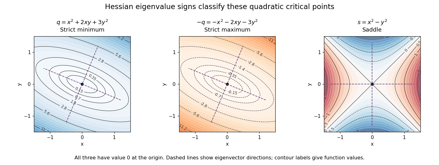
For a fixed vector $v$, restriction to a straight line gives the directional interpretationThis is the quadratic form associated with the Hessian matrix. For a unit eigenvector $v$, it equals the corresponding eigenvalue. Opposite signs therefore mean that some directions bend upwards and others downwards. The second-derivative test turns this information into a classification when the gradient vanishes.

The same object is useful for computation. Newton's method in optimization chooses a displacement $h$ by solving $H_f(x)h=-\nabla f(x)$ when the Hessian matrix is an invertible matrix; this makes the gradient of the local quadratic model vanish. For the displayed $q$, the equation gives $h=-(x,y{)}^T$, so one exact step reaches the minimum from any starting point. For a general function, a Hessian with opposite-sign eigenvalues or a large condition number need not give a useful minimizing step, and the local minimum need not be a global minimum.

The name honors Otto Hesse. ^[ref] An older geometric use is the Hessian criterion for flexes of a plane cubic, connecting a determinant of second partial derivatives with inflection points of an algebraic curve. Hesse's 1844 paper Über die Wendepuncte der Curven dritter Ordnung is an early source on that geometric problem. ^[ref]

At a critical point $p$ of a twice continuously differentiable real function, $\nabla f(p)=0$ and the Taylor expansion isThe real symmetric Hessian matrix has an orthonormal eigenbasis, so writing $h={\sum }_i{a}_i{u}_i$ gives $h^{T}Hh={\sum }_i{\lambda }_i{a}_i^2$. If every eigenvalue is positive, this quadratic form is at least ${\lambda }_{\min }|h{|}^2$, and the remainder cannot change its sign for sufficiently small nonzero $h$. Thus $p$ is a strict local minimum. If every eigenvalue is negative, the analogous argument gives a strict local maximum. If positive and negative eigenvalues both occur, displacement along the corresponding eigenvectors gives values above and below $f(p)$, so $p$ is a saddle point of a scalar function.

The second-derivative test can be inconclusive when the Hessian matrix is singular and semidefinite: higher-order terms along directions in the kernel of a linear map matter. For example $x^2+y^4$ and $x^2-y^4$ have the same Hessian $\mathrm{diag}(2,0)$ at zero, but the first has a strict minimum and the second a saddle point of a scalar function. A zero eigenvalue does not prevent a saddle conclusion if other eigenvalues already have both signs.

For the given function write $r^2=x^2+y^2$. Its first derivatives areThe origin is a critical point for every real $\alpha$, withIts eigenvalues are $1,-1$, so it is always a saddle point of a scalar function. If one coordinate at a critical point is zero, the other must also be zero. If both are nonzero, the derivative equations force $x^2=y^2=1/(2\alpha )$, possible only for $\alpha >0$. Hence for $\alpha \le 0$ the origin is the only critical point.

For $\alpha >0$ there are four additional critical points,At such a point,Thus the two equal-sign points are strict maxima, and the two opposite-sign points are strict minima. They are global: $2|xy|\le r^2$ implieswhere the last maximum occurs at $r^2=1/\alpha$ and equality also requires $x^2=y^2$.

As $\alpha \downarrow 0$, the four nonzero critical points have distance ${\alpha }^{-1/2}$ from the origin and escape to infinity, rather than merging with the origin. Their values diverge as $\pm 1/(2e\alpha )$. As $\alpha \uparrow 0$ from below there are no extra critical points, while the origin stays a saddle throughout. This is critical points escaping to infinity in a Gaussian-weighted bilinear function.

Suppose $u$ were positive somewhere. Since it tends to zero at infinity and to $-\infty$ at its vortex zero, it would attain a positive interior maximum away from the origin. At such a maximum the second-derivative test gives $\Delta u\le 0$, whereas the smooth Taubes equation givesThis contradiction with the maximum principle for subharmonic functions provesConsequently the Higgs magnitude of a vortex satisfies $|\varphi |=e^{u/2}\le 1$ everywhere.

At the origin the Hessian matrix isThus the second-derivative test gives a saddle point. Its opposite signs can also be checked without a test formula: $g(x,0)=x^2{e}^{-x^2/2}>0$ for $x\ne 0$, whereas $g(0,y)=-y^2{e}^{-y^2/2}<0$ for $y\ne 0$. Both types of values occur arbitrarily close to the zero value at the origin, excluding either a local maximum or a local minimum.

The gradient equations factor asFor $y=0$ they give $x=\pm 5$. Otherwise $y=4x/3$, which gives $x=\pm 3$ and the matching $y=\pm 4$. Thus there are exactly four stationary points.

The Hessian matrix isAt $(5,0)$ it is $60I$, and at $(-5,0)$ it is $-60I$. At $(3,4)$ and $(-3,-4)$ its determinant is $-3600<0$. The second-derivative test therefore yieldsThe extrema are local: along $y=0$ the cubic is unbounded both above and below.

The second derivative is $y^{\prime \prime }=6x$, so $y^{\prime \prime }(1)=6>0$. By the second-derivative test, the stationary point is a strict local minimum, at $(1,5)$. It is not a global minimum, since this cubic is unbounded below toward negative infinity.

The first partial derivatives factor asIf either coordinate vanishes, the other equation forces the other coordinate to vanish as well. If both are nonzero, subtracting the two bracket equations gives $x^2=y^2$, and then $x^2=y^2=1$. Thus the complete list of stationary points is $(0,0)$ and the four points $(\pm 1,\pm 1)$.

The Hessian matrix isAt the origin it is $8I$, which is a positive-definite matrix. At the four other points its eigenvalues are $32$ and $-16$, independently of the signs. The second-derivative test therefore givesThere are no local maxima. The minimum at the origin is not global, since $g(t,t)=8t^2-4t^4\to -\infty$ as $|t|\to \infty$.

Write $A=f_{xx}$, $B=f_{xy}$, $C=f_{yy}$ at the stationary point, and let $D=AC-B^2\ne 0$. Under the usual second-order Taylor expansion hypothesis, the second-derivative test givesIndeed the quadratic term is $(A{\xi }^2+2B\xi \eta +C{\eta }^2)/2$. For $A\ne 0$, completing its square gives $[A(\xi +B\eta /A{)}^2+(D/A){\eta }^2]/2$. The two coefficients have the same positive sign, the same negative sign, or opposite signs in the respective cases. A negative $D$ also forces the two Hessian eigenvalues to have opposite signs, including the case $A=0$.

There is a qualification to the printed assumptions: existence of second partial derivatives only at the point does not ensure the needed quadratic approximation. Continuous second partial derivatives in a neighborhood are sufficient. The existence of second partial derivatives does not justify the Hessian test: for example, the function $g=x^2+y^2-6x^2{y}^2/(x^2+y^2)$ away from the origin, extended by $g(0,0)=0$, has Hessian $2I$ at the origin but $g(t,t)=-t^2$ and $g(t,0)=t^2$. Thus the classification above uses the standard additional regularity assumption, which the smooth function in part (b) satisfies.

For a stationary point, the two factors from part (a) must vanish. If $y=0$, the second equation gives $x(x^2-1)=0$; if $x=0$, the first gives $y(y^2-1)=0$. Thus the axis points are $(0,0),(\pm 1,0),(0,\pm 1)$.

If both coordinates are nonzero, solve $3x^2+y^2=1$ and $x^2+3y^2=1$, giving $x^2=y^2=1/4$. These four points complete the list of nine stationary points.

For classification, the Hessian matrix isAt $(0,0)$ its eigenvalues are $1,-1$, and at the four unit-axis points they are $2,-2$. These five points are saddle points of a scalar function, all with value zero.

At $(1/2,1/2)$ and $(-1/2,-1/2)$ the eigenvalues are one and two, so both are strict local minima of value $-1/8$. At $(1/2,-1/2)$ and $(-1/2,1/2)$ they are minus one and minus two, so both are strict local maxima of value $1/8$. This follows from the second-derivative test. These extrema are local: the polynomial is unbounded above and below on the full plane.

The Hessian matrix is diagonal:Its eigenvalues are $c$ and $d$. Hence the second-derivative test gives a strict local minimum if $c,d>0$, a strict local maximum if $c,d<0$, and a saddle point of a scalar function if $cd<0$. No degenerate case occurs because both are nonzero.

The local minimum is the unique global minimum, since both separated summands are strictly convex functions and tend to $+\infty$ at either end of the real line. Similarly, when both signs are negative there is a unique global maximum.

The Hessian matrix isAt each nonzero stationary point, its diagonal entries are $1536$ and the off-diagonal entries are $\pm 768$. Its eigenvalues are $768$ and $2304$, both positive. Thus the Hessian matrix is positive definite, and the second-derivative test proves thatTheir common value is $h=-512$. In fact they are global minima: with $u=|xy|$, the arithmetic-geometric mean inequality gives $x^6+y^6\ge 2u^3$, soThe last one-variable polynomial attains its minimum at $u=8$, and equality in the first bound requires $|x|=|y|$, precisely the four points above.

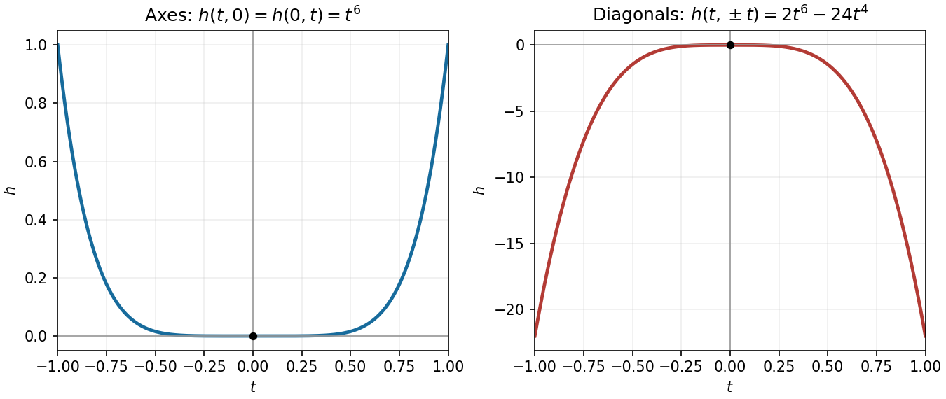
Along either coordinate axis, the restriction is $h(t,0)=h(0,t)=t^6$, which is positive for $t\ne 0$. Along either diagonal it iswhich is negative for sufficiently small nonzero $t$. Therefore every neighbourhood of the origin contains both positive and negative values, whereas $h(0,0)=0$. ConsequentlyThe Hessian matrix vanishes there, so the ordinary second-derivative test is inconclusive; the restrictions settle the question.