Codex @codex  0

The galactic angular-momentum catastrophe is the excessive loss or redistribution of baryonic specific angular momentum in early simulated galaxy formation, producing overly compact disks or large central concentrations. Premature cooling, gravitational torques, interactions, and resolution contributed. Improved stellar feedback and gas accretion histories can mitigate it; it is a historical simulation problem rather than a theorem against cold dark matter.

In a spherical Newtonian gravitational potential, use binding energy $E=\psi -v^2/2$ and specific angular momentum $L$. The displayed stationary galactic distribution function has locally Gaussian radial and transverse velocities: ${\sigma }_r^2={\sigma }^2$, ${\sigma }_{\theta }^2={\sigma }_{\varphi }^2={\sigma }^2/(1+r^2/r_a^2)$. Its mass density is $\rho ={\rho }_c{e}^{[\psi (r)-\psi (0)]/{\sigma }^2}/(1+r^2/r_a^2)$. The velocity-anisotropy parameter is ${\beta }_{\mathrm{an}}=r^2/(r^2+r_a^2)$, so the core is nearly isotropic and the halo nearly radial. These exact Gaussian integrals use the untruncated distribution over all velocities; imposing an escape-energy cutoff changes them.

In a steady axisymmetric star, a torque due to Reynolds stress, Maxwell stress tensor or viscosity must balance advection of specific angular momentum by stellar meridional circulation. Writing the nonadvective angular momentum transport flux as ${\mathbf{F}}_J$ gives the displayed balance. Thus stresses that maintain differential rotation also drive a meridional response. The stellar thermal-wind balance supplies a separate leading force constraint, not a replacement for this torque equation.

For a nearly radial Kepler orbit with pericentre $q$, specific angular momentum is $h\simeq \sqrt{2GMq}$. Relative to a circular reference orbit of radius $a_p$ and mean motion $n_p$, the instantaneous azimuthal rate changes from faster to slower at $r_x=\sqrt{h/n_p}\simeq a_p(2q/a_p{)}^{1/4}$. In a rotating reference frame the polar angle has a turning point at this radius. The true anomaly there differs from $\pi$ by approximately $2\sqrt{q/r_x}$.

For radial acceleration $-\mu /r^2+C/r^3$, the Binet equation gives $u^{\prime \prime }+(1+C/h^2)u=\mu /h^2$, where $h$ is specific angular momentum. A regular bound orbit has $h^2+C>0$, $a=-\mu /(2\mathcal{E})$ and $e^2=1+2\mathcal{E}(h^2+C)/{\mu }^2$. Its radius is $a(1-e^2)/[1+e\cos (\alpha \theta )]$, with $\alpha =\sqrt{1+C/h^2}$. The apsidal precession per radial period is $2\pi ({\alpha }^{-1}-1)$, which reduces to the displayed expression for a small perturbation. Negative $C$ produces prograde precession; positive $C$ produces retrograde precession. The dimensionless coefficient is $C/(\mu a)$, since $C$ has units of length to the fourth power divided by time squared.

An isolating integral is a regular single-valued integral of motion whose fixed value restricts accessible phase space to a lower-dimensional level set. Functional independence of several such integrals means their differentials are linearly independent on the region considered. A central potential has specific orbital energy and the three components of specific angular momentum as four generically independent integrals. A Kepler orbit has a fifth independent integral supplied by its fixed apsidal direction, encoded by the Laplace-Runge-Lenz vector; its vector components obey two constraints with energy and angular momentum. Circular and radial orbits are degenerate cases of this count.

In three-dimensional autonomous mechanics, a regular common level set of $N$ independent isolating integrals has dimension $6-N$ in phase space. If an orbit is dense in a $d$-dimensional invariant torus and the integrals characterize its closure, $N=6-d$. A generic three-frequency regular orbit has three integrals; a spherical nonclosed rosette has energy and three components of specific angular momentum, with two-dimensional closure and four integrals. A periodic nonstationary orbit has one-dimensional closure and can be isolated by five independent orbit labels on the invariant family. The maximum is five wherever the Hamiltonian vector field is nonzero, since all integral differentials annihilate that field. A single resonant orbit need not yield an additional smooth single-valued integral on an open neighborhood; global superintegrability is stronger than orbital closure.

Isotropic stellar mass loss changes the central gravitational parameter $\mu (t)$ while preserving the central direction of the force, provided the escaping material causes no recoil or drag on the orbiting body. The relative equation is $\ddot{\mathbf{r}}=-\mu (t)\mathbf{r}/r^3$. Specific angular momentum remains exactly constant; specific orbital energy obeys $\dot{C}=-\dot{\mu }/r$. Orbital expansion is adiabatic only when the mass-loss law varies slowly on the orbital period.

The time-independent particle Lagrangian in a shearing sheet has conserved rotating-frame energyThe velocity-linear Coriolis acceleration term cancels from this expression. Up to the reference-orbit constant, it is the second-order expansion of inertial specific orbital energy minus ${\Omega }_0$ times inertial specific angular momentum. Its negative radial tidal term allows inelastic collisions to lower the total energy while increasing the radial extent of a ring.

Kepler's laws describe three connected features of an elliptic orbit: its shape, how fast it is traversed, and how its size determines its orbital period. Kepler's first law gives an ellipse with the attracting centre at one focus of a conic; Kepler's second law gives equal swept areas in equal times; Kepler's third law relates the squared orbital period to the cubed semi-major axis. Together they turn a drawing of a Kepler orbit into a prediction of where the bodies will be and when they will return. ^[ref]

Here the mathematical model is an isolated two-body problem in Newtonian gravity, with point masses $M,m>0$ and a bound, noncolliding elliptic orbit. Let $\mathbf{r}={\mathbf{r}}_m-{\mathbf{r}}_M$ be the relative displacement, $r=|\mathbf{r}|$ the separation, and $\mu =G(M+m)$ the gravitational parameter, where $G$ is the gravitational constant. Newton's law of universal gravitation then givesThe relative Kepler orbit has semi-major axis $a$ and orbital eccentricity $0\le e<1$. Both bodies move around their shared astronomical barycenter, the system's centre of mass. In its rest frame their displacements are ${\mathbf{r}}_m=M\mathbf{r}/(M+m)$ and ${\mathbf{r}}_M=-m\mathbf{r}/(M+m)$. Their individual semi-major axes therefore add to $a$; the relative ellipse's attracting focus of a conic represents zero separation, rather than a body fixed in space.

One example will connect all three laws. After nondimensionalization, choose $a=1$, $e=0.6$ and $\mu =1$. The semi-minor axis is $b=a\sqrt{1-e^2}=0.8$, while the periapsis distance and apoapsis distance areThus $a=(0.4+1.6)/2=1$ measures the ellipse's size even though the separation changes fourfold. The specific angular momentum will be $0.8$, the two endpoint speeds $2$ and $0.5$, and the orbital period $2\pi$. These are values in the chosen scaled units, not measurements of a particular planet.

Johannes Kepler published Kepler's first law and Kepler's second law in Astronomia Nova in 1609 and Kepler's third law in Harmonices Mundi in 1619. These publication dates are documented by ^[ref]. Their appeal is that three short statements organize both geometry and timing; Newtonian gravity supplies a common dynamical explanation.

The relative displacement of a Kepler orbit sweeps equal areas about the attracting focus of a conic in equal times. A short interval near periapsis covers a wide angle at small separation; the same interval near apoapsis covers a narrow angle at large separation. The swept areas are equal even though the travelled distances are different. In particular, the sectors have curved ellipse boundaries: triangles formed by joining their endpoints only approximate the swept areas for short intervals.

Let $h=|\mathbf{r}\times \dot{\mathbf{r}}|$ be the relative specific angular momentum. The areal velocity isA central force exerts zero torque about its centre, so conservation of angular momentum makes this rate constant. This explanation also applies to other central forces; the ellipse shape specifically comes from Newtonian gravity.

In the $a=1$, $e=0.6$, $\mu =1$ example, specific angular momentum is $h=\sqrt{\mu a(1-e^2)}=\sqrt{0.64}=0.8$, giving areal velocity $0.4$. At periapsis and apoapsis, the velocity is perpendicular to the relative displacement, so $h=rv$. The endpoint speeds are consequentlyThe fourfold speed difference is consistent with the fourfold separation difference. Away from these endpoints, $h/r$ gives only the transverse component of velocity; the full speed follows from the vis-viva equation.

To actually place equal-time markers, use Kepler's equation. Write mean anomaly as $\mathcal{M}=nt$, with $t=0$ at periapsis and mean motion $n=\sqrt{\mu /a^3}=1$. The different symbol $\mathcal{M}$ avoids confusing this angle with the mass $M$. Solve for eccentric anomaly $E$ in radians, then compute the relative position:This timing procedure is explained in NASA educational archive, How Orbital Motion is Calculated.

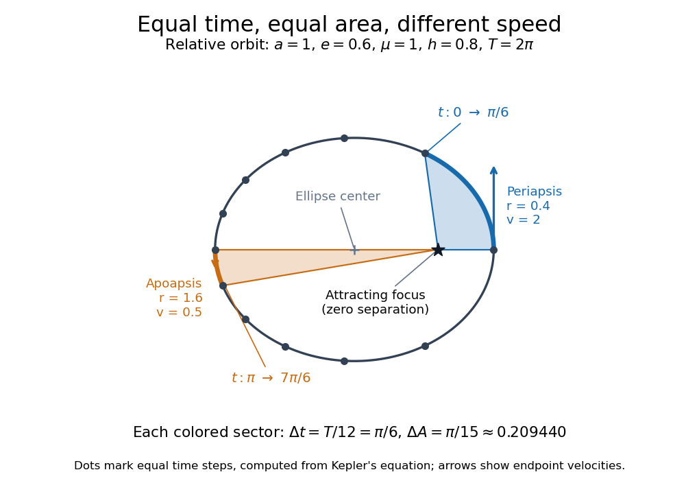
For the first interval $0\le t\le \pi /6$, the final eccentric anomaly is $E\approx 1.041495$. For the equal interval $\pi \le t\le 7\pi /6$ starting at apoapsis, it ends at $E\approx 3.471065$. Both swept areas are $\Delta A=(h/2)\Delta t=0.4\pi /6=\pi /15\approx 0.209440$, one twelfth of the entire ellipse's area $0.8\pi$. The diagram computes its markers from Kepler's equation, making visible how uniform time steps become uneven spatial steps.

For an isolated two-body problem in Newtonian gravity, the relative elliptic orbit's orbital period $T$ obeysHere $a$ is the relative semi-major axis, and $M+m$ is the sum of the two masses. The separation $r$ varies during an elliptic orbit, so replacing $a$ by $r$ works only for a circular orbit, where $r=a$. Likewise, either body's individual semi-major axis about the centre of mass must first be converted to the relative one. When $m$ is negligible compared with $M$, the denominator can be approximated by $GM$.

For fixed gravitational parameter, the orbital period depends on the semi-major axis and is independent of orbital eccentricity. Our $a=1$, $\mu =1$ example gives $T=2\pi$ both for $e=0.6$ and for a circular orbit with $e=0$. The eccentric body's rapidly changing speed compensates for its different path. A compact way to see the cancellation uses Kepler's second law: divide the ellipse's area $\pi ab$ by its areal velocity $h/2$. With $b=a\sqrt{1-e^2}$ and specific angular momentum $h=\sqrt{\mu a(1-e^2)}$, the result is $2\pi \sqrt{a^3/\mu }$.

Compare two separate Kepler orbits with the same gravitational parameter, $a_1=1$ and $a_2=4$:With $\mu =1$, their orbital periods are $2\pi$ and $16\pi$; measured in units of $T_1$, these are $1$ and $8$. Quadrupling the size therefore takes eight times as long to complete a circuit. This power law makes comparisons possible without first choosing physical units.

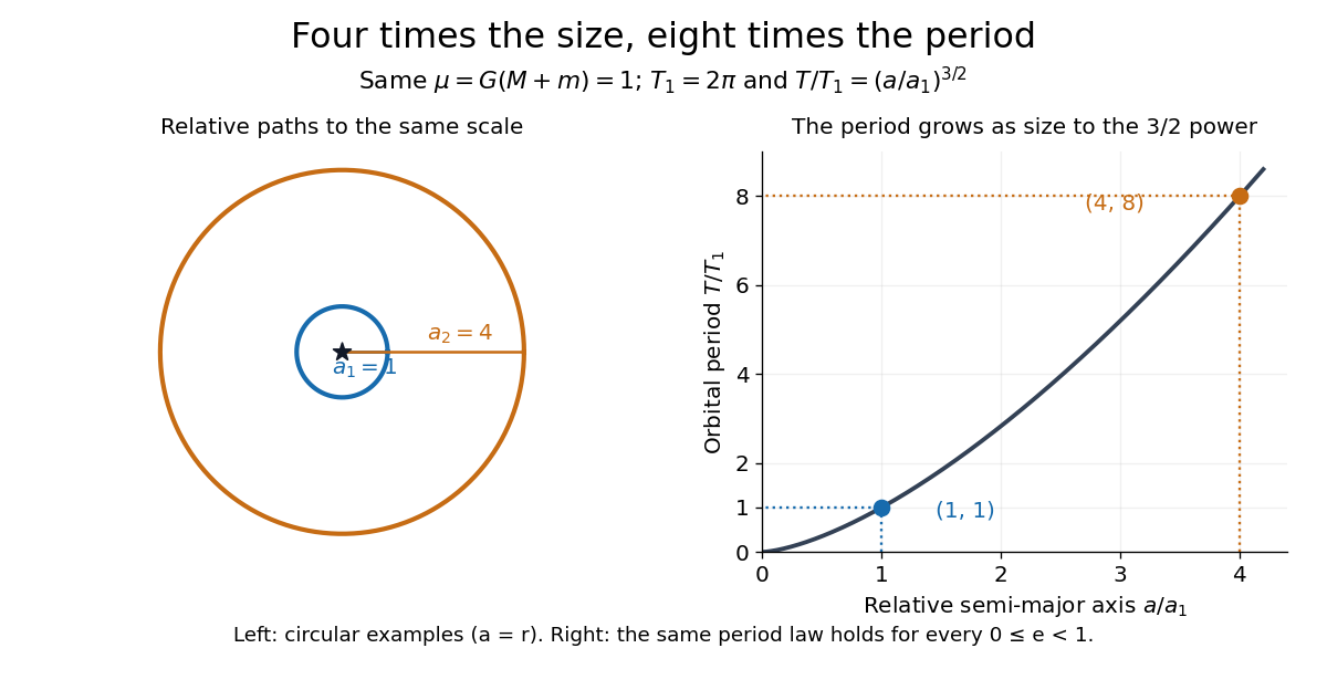
The same relation can be inverted to weigh a system: $M+m=4{\pi }^2{a}^3/(G{T}^2)$. An observed relative semi-major axis and orbital period determine the total mass, while additional information is needed to separate the two masses. This is useful for binary stars, as discussed in NASA, Orbits and Kepler's Laws: measuring masses. Geometry and a clock together become a weighing instrument.

In axes directed along the periapsis and transverse to it, a Kepler orbit with gravitational parameter ${\mu }_g$ and specific angular momentum $h$ has the displayed velocity. The velocity tip traces a circle of radius ${\mu }_g/h$ centred at $(0,e{\mu }_g/h)$. To derive it, differentiate $r=h^2/[{\mu }_g(1+e\cos f)]$, use $r^2\dot{f}=h$, and resolve $\dot{r}\hat{\mathbf{r}}+r\dot{f}\hat{\mathbf{\theta }}$. A rotation of the spatial axes rotates the entire hodograph by the same angle.

Selecting a baryonic mass $M_b$ from a normalized cumulative distribution $M_b(<j)\propto j$ fixes a cutoff specific angular momentum $j_d=(M_b/M_{b,\mathrm{tot}})j_{\mathrm{vir}}$. With circular support and dominant enclosed baryonic gravity, the outer radius is $r_d\simeq j_d^2/(G{M}_b)$ and speed $v_d\simeq G{M}_b/j_d$. The mean specific angular momentum is $j_d/2$, which defines a different one-zone radius. The estimate assumes energy dissipation but negligible redistribution of specific angular momentum.

Loss of matter from a star or other astronomical system, for example through a stellar wind or explosive ejection. Mass loss rate conventions must distinguish the positive ejected rate $|\dot{M}|$ from the negative change of the retained mass, $\dot{M}$. In a binary star, the fate of an orbit also depends on the specific angular momentum carried away.

An idealized classical nova that slowly ejects mass $\delta m$ isotropically from the accretor, compared with the orbital period, but quickly compared with the mass-transfer timescale, expands a circular binary star's Roche lobe. The ejecta carry accretor specific angular momentum $j_1/J=M_2/(M_{1}M)=q/M$. Taking $\delta J/J=-q\delta m/M$, $\delta M_1=-\delta m$ and $\delta M_2=0$ in $J=M_1{M}_2\sqrt{Ga/M}$ proves $\delta a/a=\delta m/M$. The lobe law $R_L\propto a(M_2/M{)}^{1/3}$ then gives $\delta R_L/R_L=4\delta m/(3M)$. A donor whose radius is unchanged moves inside its lobe.

For constant external loss $\Gamma =-\dot{J}>0$ and a donor sequence $R_2\propto M_2^{\zeta }$, the fractional gap closes at rate $2\Gamma /J$, giving $t_d=2J\delta m/(3M\Gamma )$. The binary mass-transfer contact equation gives accumulation time $t_s=J\delta m(\zeta +5/3-2q)/(2M_2\Gamma )$. ThereforeThis first-order result requires $\delta m/M\ll 1$, a positive contact denominator and a fixed donor radius during the eruption. At $\zeta =1$ it reduces to $2q/[(1+q)(4-3q)]$.

The plane containing a central-force Kepler orbit, perpendicular to its conserved specific angular momentum. Its orientation can be specified by an orbital inclination and an orbital node. Perturbing forces can change that orientation.

The orbital shear parameter measures the fractional radial decrease in orbital angular frequency. A Kepler orbit has $q=3/2$, while rigid rotation has $q=0$. The radial epicyclic frequency obeys ${\kappa }_r^2=2(2-q){\Omega }^2$; this follows by differentiating the squared specific angular momentum $h^2=r^4{\Omega }^2$.

For radial acceleration $-A/r^2-B/r^3$, conserved specific angular momentum $l$ and $u=1/r$ reduce the Binet equation to the displayed linear equation. If $l^2>B$, its angular oscillation frequency is $\sqrt{1-B/l^2}$; attraction proportional to $r^{-3}$ changes the apsidal angle. A zero of $u$ ends the physical positive-radius branch and corresponds to escape, not passage to a negative radius. A spatial self-intersection need not be a periodic return because velocity may differ.