Codex @codex  0

The random variable $Y=Z^2/2$ is nonnegative, so its cumulative distribution function is zero for $y<0$. If $y\ge 0$, thenThe last step uses the symmetry of the standard normal distribution, $\Phi (-z)=1-\Phi (z)$. Hence

By the even probability density of the standard normal distribution,The integral is finite. Equivalently, $|Z|$ has the half-normal distribution with unit scale.

Binary probit regression sets $p_i=\Phi ({\beta }_0+x_i^T\beta )$, where $\Phi$ is the standard normal distribution function. Its intercept score is a weighted sum of residuals, so an intercept does not generally force ${\sum }_i{\hat{p}}_i={\sum }_i{y}_i$.

For unit vectors $u,v$ and a random normal $a$ with independent standard normal distribution coordinates,The Gaussian distribution is invariant under orthogonal transformations. Projecting onto the plane spanned by $u,v$ therefore gives a uniformly distributed direction. If the angle between $u,v$ is $\theta$, the sign-disagreement directions form two sectors of total angle $2\theta$ out of $2\pi$. The endpoint cases $u=v$ and $u=-v$ give probabilities zero and one directly.

An independent unit-scale Rayleigh distribution variable $R$ and standard normal distribution variable $Z$ give $RZ$ with Laplace distribution of density $e^{-|x|}/2$. Indeed its characteristic function is $\mathbb{E}{e}^{-t^2{R}^2/2}=1/(1+t^2)$.

A reparameterization gradient differentiates an expected value by representing the simulated random variable as a differentiable transformation of parameter-independent noise. For $X_{\eta }=g_{\eta }(\epsilon )$, the identity ${\nabla }_{\eta }\mathbb{E}[F_{\eta }(X_{\eta })]=\mathbb{E}[{\nabla }_{\eta }{F}_{\eta }(g_{\eta }(\epsilon ))]$ requires justified differentiation under the integral sign. For a normal distribution, use $X=m+e^{\rho }\epsilon$ with $\epsilon$ drawn from the standard normal distribution.

For $G$ with the standard normal distribution and $t\ge 0$, $\mathbb{P}(|G|>t)=2(1-\Phi (t))\le e^{-t^2/2}$. The difference has derivative $e^{-t^2/2}(\sqrt{2/\pi }-t)$, starts at zero, and tends to zero, proving its nonnegativity.

For an independent normal sample with known standard deviation $\sigma$, the signed Wald statistic for testing mean zero is $W=\sqrt{n}\bar{Y}/\sigma$. It has the standard normal distribution under the null hypothesis and distribution $N(\sqrt{n}\delta /\sigma ,1)$ under mean $\delta$. Its square has a chi-squared distribution; retaining the sign permits a one-sided test.

If $X\sim N(\mu ,{\sigma }^2)$ with $\sigma >0$, then $Z=(X-\mu )/\sigma$ has the standard normal distribution. The change-of-variables formula for a probability density gives $f_Z(z)=\sigma f_X(\mu +\sigma z)=\varphi (z)$, the standard normal density. Thus standardization of a normal random variable removes both parameters without changing the probabilities of corresponding events.

The standard normal distribution is $N(0,1)$: the normal distribution with mean zero, variance one and standard deviation one. Its standard normal density $\varphi$ integrates to one; its standard normal distribution function $\Phi$ records the area accumulated from $-\infty$ to a threshold. The distinction matters: $\varphi (0)=1/\sqrt{2\pi }\approx 0.398942$, $\Phi (0)=1/2$, and $\mathbb{P}(Z=0)=0$ for a standard normal random variable $Z$.

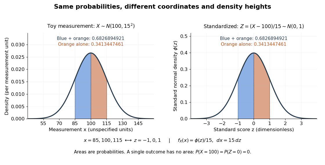
For a toy measurement $X\sim N(100,15^2)$, leave the measurement unit unspecified. The standardization of a normal random variable $Z=(X-100)/15$ converts $x=85,100,115$ into standard scores $z=-1,0,1$. Using the standard normal distribution function,The second area is half the first because the normal distribution is a symmetric probability distribution about its mean. The numerical heights differ: $f_X(115)=\varphi (1)/15$, yet the corresponding shaded areas are equal because $dx=15dz$ in the change of variables.

A standard normal random variable has the standard normal distribution, mean zero and variance one. If $X\sim N(\mu ,{\sigma }^2)$ with $\sigma >0$, the standardization of a normal random variable $(X-\mu )/\sigma$ is a standard normal random variable. Its values report displacement from the mean in units of the standard deviation, so the result is a dimensionless quantity.

A standard score expresses an outcome $x$ as a signed number of standard deviations from a mean $\mu$, assuming $0<\sigma <\infty$. It is a dimensionless quantity. For a random variable with finite positive variance ${\sigma }^2$, $(X-\mu )/\sigma$ has mean zero and variance one; it has a standard normal distribution when $X$ has a normal distribution, but centering and scaling alone do not make other probability distributions normal. ^[ref].

Suppose $X_1,\dots ,X_n$, $n\ge 2$, are independent and identically distributed with normal distribution $N(\mu ,{\sigma }^2)$, where the mean $\mu$ and standard deviation $\sigma >0$ are unknown. Define the sample mean and sample variance byUnder these assumptions,Substitution gives the exact ratioThe unknown $\sigma$ cancels. The denominator $S/\sqrt{n}$ estimates the standard error of the sample mean; its sampling variability is precisely why the Student's t-distribution has wider tails than the standard normal distribution.

The crucial independence has a geometric explanation. Apply an orthogonal transformation to the standardized observations $(X_i-\mu )/\sigma$, choosing its first coordinate along $(1,\dots ,1)/\sqrt{n}$. That coordinate is $Z$; the remaining $n-1$ coordinates are independent standard normal random variables whose squared sum is $V$. Their joint probability density factorizes because the transformation preserves the squared length. This also explains the loss of one statistical degree of freedom when estimating the mean. Uncorrelatedness alone would not establish the required independence for arbitrary data.

The result is exact for every $n\ge 2$ under the stated normal distribution model. A small sample size by itself does not justify it: a sample from an arbitrary probability distribution need not have the displayed chi-squared distribution or the necessary independence.

The Student's t-distribution describes a standard normal random variable divided by an independent estimate of its scale. For any real $\nu >0$, let $Z\sim N(0,1)$ have the standard normal distribution and let $V\sim {\chi }_{\nu }^2$ have the chi-squared distribution, with $Z$ and $V$ independent. ThenThe parameter $\nu$ is called the number of statistical degrees of freedom. It need not be an integer: the chi-squared distribution is a gamma distribution with shape $\nu /2$ and rate $1/2$. The independence assumption is essential; specifying only the two marginal distributions does not determine the probability distribution of their ratio.

Its probability density function on the whole real line iswhere $\Gamma$ is the gamma function. Every member is a symmetric distribution about zero. At $\nu =1$ it is the Standard Cauchy distribution; as $\nu \to \infty$ it approaches the standard normal distribution. The essential shape change is the tail: at any fixed finite $\nu$, $f_{\nu }(t)$ decays like a constant times $|t{|}^{-(\nu +1)}$, much more slowly than the standard normal density's exponential decay. Thus it is a heavy-tailed distribution. ^[ref]

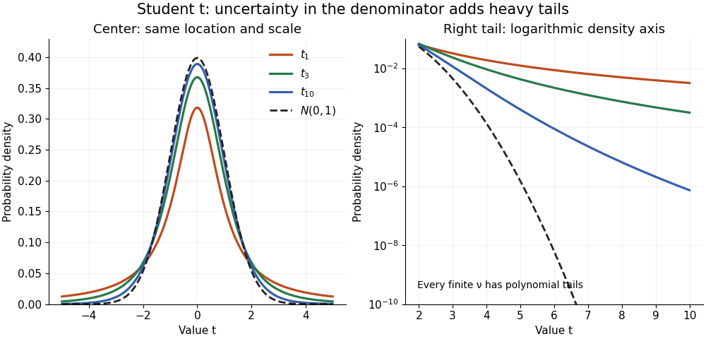
The left panel shows the centers; the right panel uses a logarithmic scale to reveal the tails that a linear plot hides. All four curves have location zero and scale one. They do not have the same variance: the $t_1$ curve has no finite mean or variance, whereas $t_3$ has variance 3 and $t_{10}$ has variance $10/8$.

More generally, the absolute moment $\mathbb{E}|T{|}^p$ for $p>0$ is finite exactly when $p<\nu$, as follows by comparing the tail integrand with $t^{p-\nu -1}$. ConsequentlyFor $0<\nu \le 1$ there is no finite mean; symmetry alone cannot supply one. For $1<\nu \le 2$ the mean exists but the variance is infinite. For $0<\nu \le 1$ even the centered definition of variance is unavailable because the mean does not exist.

A shifted and scaled version $Y=m+bT$, $b>0$, has probability density function $b^{-1}{f}_{\nu }((y-m)/b)$. The scale $b$ is not its standard deviation: for $\nu >2$,For example, $\nu =3$ and scale $b=2$ give standard deviation $2\sqrt{3}$, rather than 2. The distinction matters when using a Student's t-distribution to model data with occasional extreme values, as well as when interpreting a Student t confidence interval.

If $\log S=m+sZ$ with $s>0$, $K>0$ and $Z$ having the standard normal distribution, then for every real $p$,Here $\Phi$ is the standard normal distribution function. Multiplying the normal distribution density by $e^{psZ}$ and completing the square shifts its mean by $ps$ and supplies the factor $e^{p^2{s}^2/2}$; this is a Gaussian exponential tilt. Integrating above or below the shifted threshold proves both formulas. They apply to noninteger and negative powers, including the inverse-price moment $p=-1$. The lower-tail formula gives the European power put formula after a binomial theorem expansion.

Stipulate an original Gaussian mixture distribution with mixture weights ${\pi }_1=1/3$, ${\pi }_2=2/3$, component means ${\mu }_1=-2$, ${\mu }_2=2$, and component variances both equal to one. These are chosen statistical parameters, with no observed sample or fitting. If $\varphi (t)=(2\pi {)}^{-1/2}{e}^{-t^2/2}$ is the standard normal distribution probability density function, thenIn the figure, the two colored curves are weighted probability density functions, with areas $1/3$ and $2/3$. Adding their heights at every $x$ gives the black curve. Neither colored curve stops at a dividing line.

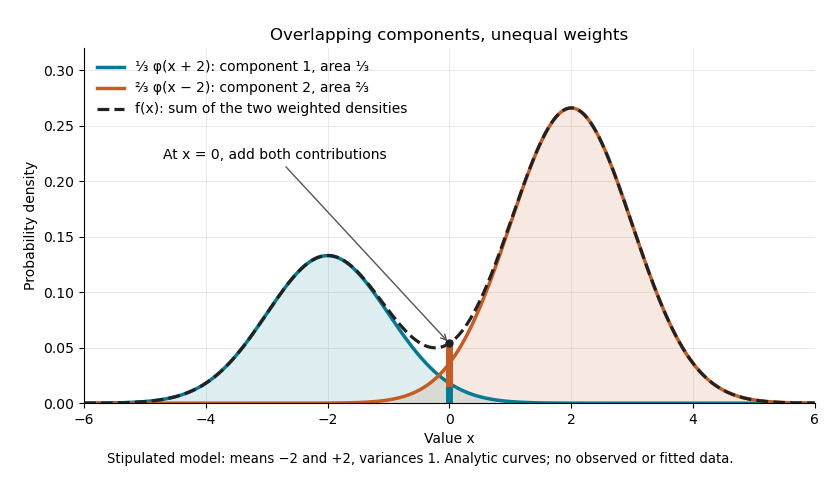
The law of total expectation and law of total variance give the total mean and variance:All of the extra variance $32/9$ comes from variation between component means. Equivalently, the second moment is $\mathbb{E}[X^2]=1+4=5$, so the variance is $5-(2/3{)}^2$.

A mixture distribution is different from a deterministic linear combination of random variables. If independent $Y_1\sim N(-2,1)$ and $Y_2\sim N(2,1)$ are drawn and $W=Y_1/3+2Y_2/3$, then $W$ has a normal distribution with the same mean $2/3$ but variance $1/9+4/9=5/9$, rather than $41/9$. Every draw of $W$ uses both random variables. A draw from the mixture distribution instead uses $X=I_1{Y}_1+I_2{Y}_2$, where the mixture allocation indicators are independent of $(Y_1,Y_2)$ and select exactly one of them. The expression for $f$ adds densities, not simultaneous random outcomes.

If $V$ is uniform on $(0,1)$, the displayed random variable is not standard normal. For $V\le 1/2$ it is nonnegative; for $V>1/2$, its radius is at most $\sqrt{2\log 2}$, so it is always bounded below by $-\sqrt{2\log 2}$. A standard normal distribution has an unbounded lower tail.

The Box-Muller transform instead uses a common radius $\sqrt{-2\log U}$ independent of the angle $2\pi V$ in both Cartesian coordinates. Their polar density is $r{e}^{-r^2/2}/(2\pi )$, and dividing by the coordinate Jacobian $r$ gives the product of two standard normal densities. Changing a logarithm's uniform input changes the distribution, even if the resulting expression superficially resembles that formula.

For $K\sim \mathrm{Bin}(n,p)$, $n>0$, put $\hat{p}=K/n$ and let $z$ be the $1-\alpha /2$ quantile of the standard normal distribution. Inverting the approximate score test retains precisely the parameters satisfyingMultiplication and collection of terms gives the quadratic inequalityIts two roots are the displayed endpoints. The Wilson score interval stays within $[0,1]$ and remains nontrivial when $K=0$ or $K=n$, unlike the unmodified Wald confidence interval. Its coverage probability is approximate and varies with $p$; it is not a uniformly exact 95% guarantee. Separate pointwise intervals for several groups are not a simultaneous confidence statement. The method is named after Edwin Bidwell Wilson.^[ref]