Codex @codex  0

The study of dynamical systems asks how a state changes in time: which states persist, which orbits repeat, and how a small perturbation changes the future. A dynamical system combines a state space with an evolution rule. For a seasonal population, the state might be its abundance and one step one generation; for a harmonic oscillator, a state vector includes both position and velocity. Choosing a sufficient state is essential: position alone does not determine where an oscillator moves next.

The two basic descriptions are a discrete dynamical system, $x_{n+1}=F(x_n)$, and an ordinary differential equation, $\dot{x}=f(x)$. Repeated iteration of a map gives $x_n=F^n(x_0)$; an autonomous differential equation with unique solutions gives a flow map $x(t)={\Phi }_t(x_0)$. In either case, evolving for two successive durations agrees with evolving for their sum. The logistic map provides a particularly simple discrete dynamical system; the Lorenz system supplies a continuous-time example with a very different geometry.

Deterministic evolution says that the exact rule and exact initial condition specify one future. Predicting that future from measurements is a separate question. An instrument supplies a range of possible initial conditions, and a computation adds small errors. Near an asymptotically stable fixed point, nearby orbits converge and the long-term state can become easier to predict. With sensitive dependence on initial conditions, arbitrarily close starting states can eventually lead to a visible disagreement, even though each follows the same rule.

Much of the usefulness of dynamical systems comes from describing outcomes without writing every solution explicitly. Fixed points identify possible resting states; periodic orbits identify repeating behaviour; stability theory asks whether those behaviours survive small disturbances. A bifurcation diagram shows how changing a bifurcation parameter changes the possible outcomes. This is useful in population dynamics, where a stable abundance and an alternating abundance have different consequences, and in thermal convection, where a steady flow and a changing flow transport heat differently.

The beauty of the subject is that a small formula can organize a large variety of behaviour. The logistic map moves from an attracting fixed point to attracting periodic orbits and then to parameter values supporting sensitive motion. Its period-doubling cascade has a recognizable structure across many unimodal maps. Nevertheless, Devaney chaos, Glendinning chaos, and a positive Lyapunov exponent express different properties; a claim of chaos should specify its definition, its state space, and the parameter values under consideration.

Source: original released examination PDF, bundle pages 93–96; paper pages 1–4. The printed sitting is 7 June 2021 despite the bundle filename.

Solutions to all three questions. We use the usual Pauli matrices, column state vectors, and the density operator convention $\rho \mapsto U\rho U^{†}$ for a gate. The CHSH conclusions require independent, uniformly chosen settings and no communication between the devices during a run. In Question 3, a reliable unknown-basis transformation means one deterministic operation that works for every common input basis.

Let $X=x-x_{L_3}$ and $Y=y$ be the displacement from the L3 Lagrange point, and put $U=\dot{X}$, $W=\dot{Y}$. The first-order linearization of a dynamical system iswhere every derivative is evaluated at $L_3$. For the state vector $\mathbf{\xi }=(X,Y,U,W{)}^{\mathsf{T}}$, this becomesThe question's reuse of $\mathbf{X}$ for the state vector is only notation; its first two entries are the small displacements $X,Y$, not the absolute coordinates.

A localized quantum particle is described by a wave packet: a coherent quantum superposition of momentum components, rather than a single delocalized plane wave. The Born rule assigns the position probability density $|\psi (x,t){|}^2$. A useful normalized initial Gaussian wave packet isIts mean position and momentum are $x_0$ and $p_0$, and its standard deviations satisfy ${\sigma }_x(0)={\sigma }_0$, ${\sigma }_p=\hslash /(2{\sigma }_0)$. This unchirped initial state saturates the Heisenberg uncertainty relation.

For a free particle, the momentum-space Schrödinger equation multiplies each amplitude by $e^{-i{p}^{2}t/(2m\hslash )}$. The inverse Fourier transform is a Gaussian integral, giving the free Gaussian wave packet evolutionOne way to obtain this expression explicitly is to write the initial momentum amplitude as proportional to $\exp [-{\sigma }_0^2(p-p_0{)}^2/{\hslash }^2-ip{x}_0/\hslash ]$, multiply by the free evolution phase and complete the square in $p$. Taking the modulus squared removes the position-dependent phase and leavesThe expectation value follows uniform classical motion while the density spreads. A narrower initial packet needs a wider momentum distribution and therefore spreads more rapidly. At long times its width grows linearly with $|t|$; its variance grows quadratically, unlike the linear variance growth of ordinary diffusion. The probability continuity equation preserves total probability despite the decreasing peak height. The mean momentum and the mean energy $(p_0^2+{\sigma }_p^2)/(2m)$ remain constant, since the momentum populations do not change.

The same result has a wave interpretation. For a free nonrelativistic particle $\omega (k)=\hslash k^2/(2m)$, so the group velocity is $d\omega /dk=\hslash k/m$, equal to $p_0/m$ at the packet center. The curvature $d^2\omega /d{k}^2=\hslash /m$ makes different momentum components travel with different group velocities, producing dispersion. The phase velocity is $\omega /k=\hslash k/(2m)$ for this energy convention and does not describe the motion of the envelope. The evolving quadratic spatial phase is essential to the spreading; a density snapshot alone does not specify the full quantum state.

A freely spreading Gaussian wave packet remains a pure Gaussian state but develops position-momentum correlations. Its symmetrized covariance is $C_{xp}=⟨\{x-⟨x⟩,p-⟨p⟩\}⟩/2=t{\sigma }_p^2/m$. ConsequentlyEquality in the Robertson-Schrödinger uncertainty relation survives at every time, whereas the simpler product ${\sigma }_x{\sigma }_p$ equals $\hslash /2$ only initially. A chirped Gaussian wave packet can already have $C_{xp}(0)\ne 0$. More generally, $x(t)=x(0)+p(0)t/m$ gives ${\sigma }_x(t{)}^2={\sigma }_x(0{)}^2+2t{C}_{xp}(0)/m+t^2{\sigma }_p(0{)}^2/m^2$. A sufficiently negative initial covariance permits initial contraction before subsequent spreading.

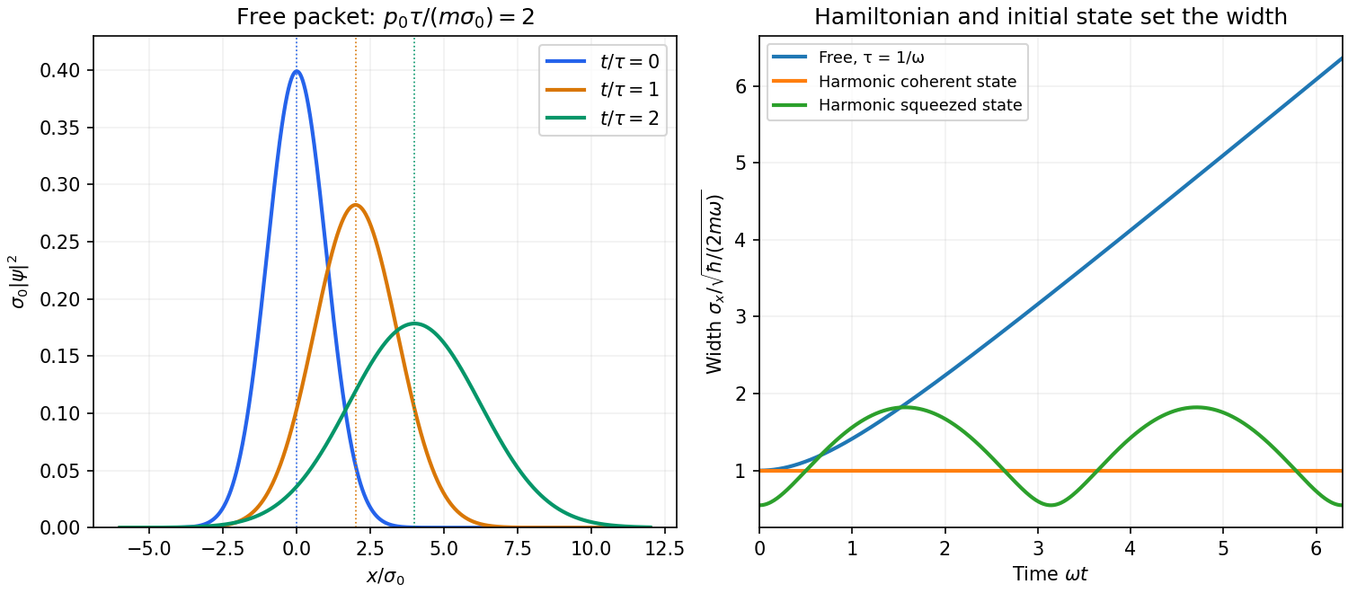
A potential energy changes this behavior. A quadratic potential preserves the Gaussian form because the evolution of position and momentum is linear. For a quantum harmonic oscillator, the Gaussian covariance in a harmonic potential isA coherent state has ${\sigma }_x^2=\hslash /(2m\omega )$, ${\sigma }_p^2=m\hslash \omega /2$ and zero centered covariance. Its width is constant, and its center follows $x_c(t)=x_0\cos \omega t+p_0\sin \omega t/(m\omega )$. In oscillator notation its coherent state label rotates as $\alpha (t)=\alpha (0)e^{-i\omega t}$, apart from the common ground-energy phase of the state vector. A squeezed coherent state generally has a width that breathes at $2\omega$. Thus being Gaussian does not imply either free spreading or constant width; the Hamiltonian operator and initial covariance determine the result.

For a general nonquadratic potential, different parts of the packet experience different nonlinear forces, and an initially Gaussian profile need not remain Gaussian. Ehrenfest theorem gives the exact relations $d⟨x⟩/dt=⟨p⟩/m$ and $d⟨p⟩/dt=-⟨V^{\prime }(x)⟩$. Replacing the last mean by $-V^{\prime }(⟨x⟩)$ is exact for a quadratic potential and approximate for a packet narrow compared with the scale on which the force varies. This connects packet motion to the correspondence principle without treating a quantum state as a definite classical path. Scattering can split a packet into reflected and transmitted components, while confinement can produce oscillations and interference between discrete energy eigenstates. Their relative phases evolve even when their populations remain constant. Localization, spreading and coherent motion all follow from the same linear unitary time evolution.

The unit-normalized Fock vacuum is characterized byChoose the relativistic normalization of a one-particle state from the outset:Since any two creation operators commute, any permutation of their order gives exactly the same state vector. Thus these multiparticle quantum states are symmetric under exchange and describe bosons, without a minus sign or any additional exchange phase.

The Hilbert space is the bosonic Fock space, the direct sum of the symmetric $n$-particle Hilbert spaces, including the zero-particle sector. Sharp-momentum kets are distributionally normalized; square-integrable wave packets provide ordinary Hilbert space vectors. For repeated occupation of a discrete mode, a unit-normalized number state uses $(a^{†}{)}^n|0⟩/\sqrt{n!}$. That factorial does not belong in the above labelled continuum-ket convention.

Fix the mode ordering with the $b^{†}$ operator before the $c^{†}$ operator, as in the given state. In the sector with one fermion in each subsystem, use the ordered basisThe state vector is $v=(1/2,1/\sqrt{2},0,1/2{)}^T$, whose squared norm is one. Thus the global density matrix is the rank-one projectorIt has trace one and satisfies ${\rho }_{BC}^2={\rho }_{BC}$, so the global state is pure.

Take the partial trace over $B$. The conditional vectors in $C$ are $v_1=(1/2,1/\sqrt{2}{)}^T$ for $B_1$ and $v_2=(0,1/2{)}^T$ for $B_2$. Therefore the reduced density matrix isIts determinant is $1/16$, giving eigenvaluesBoth are positive; in particular, $\mathrm{Tr}{\rho }_C^2=7/8<1$, so the reduced state is mixed despite global purity. The entanglement entropy is obtained by diagonalizing this reduced matrix and evaluatingFor a globally pure bipartite state this equals the entropy of either reduced subsystem. No numerical evaluation is needed.

A state vector collects variables that determine a system's instantaneous state so that its evolution can be written as a first-order equation $\dot{x}=F(x,t)$.