Codex @codex  0

A two-phase diffusion model with constant properties has similarity solutions built from the complementary error function in each half-line. Equilibrium gives $T_a=-m{C}_a$ and $C_s(a)=k_D{C}_a$. The Stefan condition and interfacial solute balance determine $\lambda$ and $C_a$; finite diffusion on both sides must be retained when constructing the narrow transition near $\lambda =0$.

For an ice layer between freshwater and cold brine, set $ϵ=\sqrt{D/\kappa }$ and use solutal similarity positions $a=2{\lambda }_a\sqrt{Dt}$, $b=2{\lambda }_b\sqrt{Dt}$. A linear ice temperature, two Stefan conditions and interfacial salt conservation determine both negative interface constants. As $ϵ\to 0$ with fixed latent-to-sensible heat ratio $S$, ${\lambda }_b=O(1)$ but ${\lambda }_a=O({ϵ}^{-1})$. Freezing above occurs over the thermal diffusion scale, while dilution-driven melting below has the much shorter solutal scale.

In a constant-thickness laminar boundary layer at an ablating glacier, approximate fluxes by $\kappa (T_{\infty }-T_i)/\delta$ and $D(C_{\infty }-C_i)/\delta$. Neglect solid diffusion and sensible heating relative to latent heat. With ablation speed $U>0$, solute balance gives $U(C_i-C_s)=D(C_{\infty }-C_i)/\delta$, so $C_i=C_s+(C_{\infty }-C_s)/(1+P)$, $P=U\delta /D$. The liquidus $T_i=T_m-\Gamma (C_i-C_s)$ and Stefan condition $UL/c_p=\kappa (T_{\infty }-T_i)/\delta$ then give the displayed law, where $A_T=LD/(c_p\kappa )$. Its positive root exists when the ocean is above its own freezing point. In the small-$P$ regime, interface salinity approaches ocean salinity; in the large-$P$ regime it approaches the ice composition.

Freezing is a liquid-to-solid phase transition. A moving phase boundary releases latent heat; its rate is constrained by heat transport and the Stefan condition. In a solution the liquidus depends on composition, so being below the pure solvent's melting temperature does not imply that the solution must freeze.

Retaining perturbation thermal diffusion givesThe displaced interfacial temperature and Stefan condition give the displayed implicit dispersion relation. In the capillarity-free limit its growing branch is exactly $\sigma =V\alpha$, which checks the limits of the small-wavelength thermal approximation for a solidification front.

Combine the full quasi-steady Stefan condition above with $\delta T=T_m{p}_T/(\rho L)$, $a=(A/(6\pi p_T){)}^{1/3}$ and the Darcy flow law to obtain an implicit pressure-growth system. Even when latent heat is negligible, a conductivity ratio $K_s/K_l=r$ changes the leading molecular driving pressure by $r^{3/4}$. Thus a reduced equal-conductivity formula requires an explicit material and rate approximation.

In a planar no-flow model with pure ice, a stable cold brine below freshwater can support an ice layer whose upper phase boundary freezes freshwater while its lower boundary melts into diluted brine. Heat conduction and salt diffusion obey different similarity scales. Local liquidus equilibrium, salt conservation and two Stefan conditions determine both boundary positions. The heat lost into the brine supports net ice growth even while some basal ice melts.

An icicle ripple is a corrugation of the ice-water interface produced while a thin flowing water film freezes. Coupling lubrication theory, surface tension, thermal conduction, and the Stefan condition determines its growth and migration.

The Maykut-Untersteiner model is a seasonally forced one-dimensional sea ice thermodynamics model with snow and saline ice layers. It couples radiative and turbulent surface fluxes, heat conduction, interior shortwave absorption, brine-dependent effective heat capacity and conductivity, snowfall, and a basal Stefan condition driven by prescribed ocean heat flux. Its annual sea-ice thermodynamic equilibrium is a periodic cycle with zero net yearly thickness change. The snow insulation and summer ice protection mechanisms compete, so additional snow need not reduce annual equilibrium thickness. The transient temperature profile need not be linear.

A shallow current receiving meltwater over its wetted area obeys $h_t+q_x=s_m$, with $q=-D{h}^2{h}_x$. The source is zero ahead of the advancing front. The Stefan condition determines normal ice-retreat speed $v_m$; the water-volume source is $s_m=({\rho }_i/{\rho }_w)v_m$, or simply $v_m$ in the equal-density approximation. Water volume and geometric excavation must be distinguished if densities differ.

The Neumann solution places a planar phase boundary at $h(t)=2\lambda \sqrt{\kappa t}$. Similarity reduction of the heat equation gives temperature profiles in terms of the error function, while the Stefan condition determines $\lambda$ implicitly.

Use undercooling $\Delta T=T_m-T_{\infty }$, solidification attachment mobility $\mathcal{M}$, velocity scale $U_0=\mathcal{M}\Delta T$, length $\ell =\kappa /U_0$ and time $\kappa /U_0^2$. Let $S=L/(c_p\Delta T)$ be the latent-to-sensible heat ratio, $\theta =(T-T_{\infty })/\Delta T$, and $\Gamma ={\gamma }_T/(\Delta T\ell )$. In the one-sided liquid-diffusion model, a travelling planar front has $\theta =S{e}^{-V\xi }$ and $V=1-S$. For a corrugation $\zeta e^{\sigma t+i\alpha y}$, the decaying thermal perturbation is $A_1{e}^{-p\xi }$, with $p^2-Vp=\sigma +{\alpha }^2$ and the branch $p=[V+\sqrt{V^2+4(\sigma +{\alpha }^2)}]/2$. The displaced kinetic condition gives $A_1=(SV-\sigma -\Gamma {\alpha }^2)\zeta$. The displaced Stefan condition gives $S\sigma \zeta =p{A}_1-S{V}^2\zeta$. Eliminating $A_1$ proves the displayed dispersion relation. Neglect of solid-side perturbation heat flux is part of this model.

Write $H=L/c_p$, $k=\rho c_p\kappa$ and $ϵ=\sqrt{D/\kappa }$. The requested model neglects density differences and uses the same thermal transport coefficients in the interfacial balances. Let $C_b=C(b(t),t)$ and $T_b=T_m-m{C}_b$. With no imposed heat gradient in the fresh liquid, its temperature remains $T_m$. The prescribed linear temperature in the ice isThe salt and temperature fields in the lower liquid satisfy diffusion equations, $C_t=D{C}_{zz}$ and $T_t=\kappa T_{zz}$. For constant interfacial values and the proposed similarity solution, their decaying solutions areThese follow by substituting a variable $z/(2\sqrt{\chi t})$ into the diffusion equation, which gives $U^{\prime \prime }+2\eta U^{\prime }=0$; integrating gives the complementary error function. Their values at $b$ and at infinity give the required boundary data.

For the upward-moving fresh-water/ice boundary, the Stefan condition is $\rho L\dot{a}=k{T}_{i,z}$: negative $\dot{a}$ means fresh water freezes. At the lower boundary the signed heat balance isSalt cannot enter the pure ice. With no bulk liquid motion its interfacial conservation law isThe derivatives and interface velocities areDefine $F(x)=\sqrt{\pi }x{e}^{x^2}\mathrm{erfc}x$. Substitution into all three balances givesTogether with $T_b=T_m-m{C}_b$, these determine the interfacial constants. In particular $C_b=C_0/[1-F({\lambda }_b)]$.

The physical branch has ${\lambda }_a<{\lambda }_b<0$. Since $F$ is negative at negative arguments, the salt relation gives $0<C_b<C_0$: lower-surface melting dilutes the brine. Combining the two heat balances eliminates the ice gradient and givesThus $T_m>T_b>T_{\infty }>T_L(C_0)$. The interface is at local liquidus equilibrium with diluted brine, while the undiluted far-field brine remains above its own liquidus. The similarity model describes a layer starting with zero thickness, or the long-time limit when an initial finite thickness no longer sets the dominant scale.

For the small-diffusivity-ratio limit, put $A=ϵ{\lambda }_a$ and $\Delta =T_m-T_{\infty }$, keeping $S=H/\Delta$ and the imposed concentrations fixed. Seek $A=O(1)$ and ${\lambda }_b=O(1)$. Then $F(ϵ{\lambda }_b)\sim \sqrt{\pi }ϵ{\lambda }_b$ and ${\lambda }_b-{\lambda }_a\sim -{\lambda }_a$. The upper heat balance givesIn the lower balance the two terms of order ${ϵ}^{-1}$ must cancel, givingConsequentlyand $T_b-T_{\infty }\sim -\sqrt{\pi }HA$. Adding the two temperature differences yields $2A^2-\sqrt{\pi }A=1/S$. The negative root isThe resulting $C_b=(T_m-T_b)/m$ lies strictly between zero and $C_0$. The salt relation therefore determines a finite negative ${\lambda }_b$, confirming its $O(1)$ scaling. The top interface travels on the thermal scale $\sqrt{\kappa t}$, whereas the lower melting interface travels on the shorter solutal scale $\sqrt{Dt}$. This is the brine-ice sandwich with disparate diffusion scales; $S$ is the latent-to-sensible heat ratio, the reciprocal of the usual sensible-to-latent Stefan number convention.

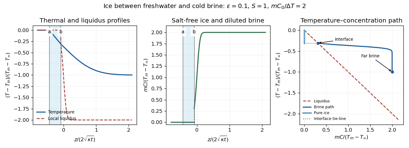
The sketches show constant fresh-water temperature, a declining linear ice temperature, and a much broader thermal than solutal boundary layer in the brine. Concentration is zero in freshwater and pure ice, jumps to $C_b$ across the lower interface, and rises to $C_0$. Accordingly the local liquidus is $T_m$ on the salt-free side, jumps to $T_b$ and falls rapidly to $T_L(C_0)$. In the phase diagram, the brine starts on the liquidus at $(C_b,T_b)$ and ends above it at $(C_0,T_{\infty })$; the pure ice has concentration zero, and the interface tie-line joins it to the diluted brine.

Physically, the cold saline liquid permits freshwater to freeze above, but salt lowers the liquidus and allows the existing ice to melt into brine below even though that brine is colder than $T_m$. Dilution raises the lower interfacial freezing temperature. Heat released by upper freezing supplies the lower melting and the conductive loss to the colder deep brine. With $|{\lambda }_a|\gg |{\lambda }_b|$, upper freezing exceeds lower melting and the ice layer thickens as $b-a\propto \sqrt{t}$.

Let the surface advance downwards at speed $V>0$. Ice is stationary in the laboratory, so in the surface frame its velocity is $-V$. The steady heat equation with volumetric heating is thereforeTake the atmospheric heat flux to be negligible in the stated model. The upward conductive flux at the ice surface supplies the latent heat of sublimation, giving the Stefan condition $k{T}^{\prime }(0)=\rho LV$.

Write $p=V/\kappa$ and $\Delta =T_s-T_{\infty }$. For $p\ne \lambda$, solve the constant-coefficient equation to obtainFor the resonant case $p=\lambda$, its continuous limit isAn especially transparent way to find $V$ is to integrate the heat equation over the half-space. Its far-field gradient vanishes, soUsing the surface heat balance givesAbsorbed radiation supplies both the latent heat and the sensible heat needed to bring incoming cold ice to the surface temperature. This is the radiatively heated sublimation profile.

The surface gradient isThus temperature first rises into the solid, but ultimately falls to the colder far field: it has a subsurface maximum. For a useful dimensionless form, set $x=\lambda z$, $r=p/\lambda$ and $S=L/(c_p\Delta )$. Thenwith limit $[1+(S+1)x]e^{-x}$ when $r=1$. The maximum is at $x_{\ast }=[\log ((rS+1)/(S+1))]/(r-1)$, or $S/(S+1)$ at $r=1$.

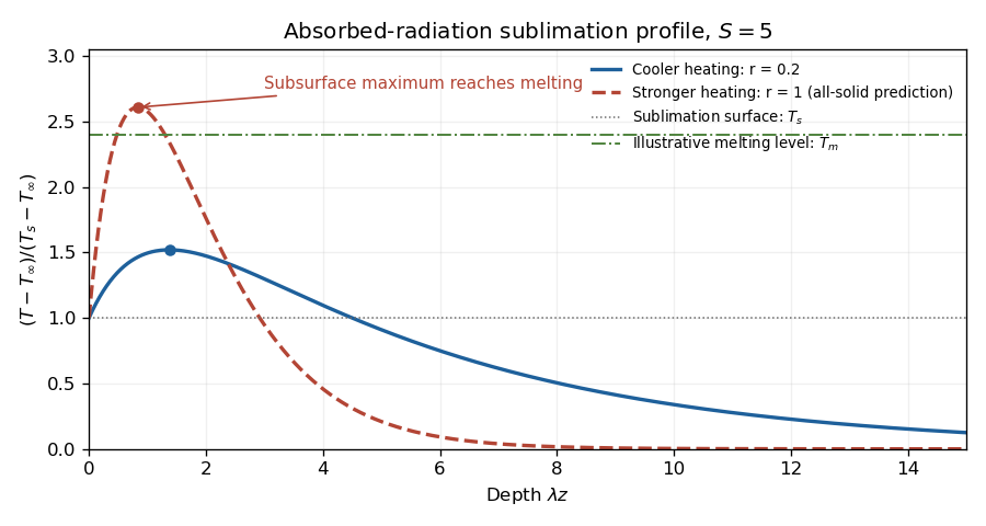
Melting begins below the surface if the interior maximum reaches $T_m$. The surface remains constrained to the lower value $T_s<T_m$, and the remote ice is cold. Increasing absorbed heating can raise the interior maximum to the melting point, after which an all-solid steady solution is no longer valid and an internal melt region must be modeled. The maximum, rather than the far-field temperature or surface temperature alone, decides onset.

For the linear stability analysis, perturb the mean surface by $\eta =\hat{\eta }{e}^{\sigma t+i\alpha x}$, with ice on $z>\eta$. Approximate the base temperature locally by $T_s+Gz$. The prescribed radiative source has no perturbation, so the perturbation heat equation is homogeneous. Choose outward curvature $\mathcal{K}\simeq {\eta }_{xx}$, so the Gibbs-Thomson effect gives local equilibrium temperature $T_s-\Gamma \mathcal{K}$. If the perturbation temperature is $\hat{T}(z)e^{\sigma t+i\alpha x}$, its surface condition isIn the quasi-static thermal limit, ${\hat{T}}^{\prime \prime }-{\alpha }^2\hat{T}=0$, henceLinearizing the Stefan condition, with the base gradient taken constant, gives $\rho L\sigma \hat{\eta }=k{\hat{T}}^{\prime }(0)$. ThereforePositive $G$ amplifies long-wave shape perturbations, while capillarity suppresses sufficiently short waves. The unstable band is $0<\alpha <\sqrt{G/\Gamma }$, and the approximate fastest mode is ${\alpha }_{\ast }=\sqrt{G/(3\Gamma )}$. This is the sublimation-front capillary instability.

The qualifications on wavelength matter. Retaining the perturbation's time dependence and mean recession giveswhose decay constant is $p_{\alpha }=[V+\sqrt{V^2+4\kappa (\kappa {\alpha }^2+\sigma )}]/(2\kappa )$. Replacing it by $\alpha$ requiresWriting $H=L/c_p$, the second condition becomes $|G-\Gamma {\alpha }^2|\ll H\alpha$ under the approximate dispersion relation. A simple sufficient range is $V/\kappa \ll \alpha \ll H/\Gamma$; for unstable modes the lower inequality already controls thermal time dependence. Large $S$ alone does not justify arbitrarily small $\alpha$.

Finally the local linear background is appropriate only if the perturbation penetration depth is shorter than its curvature length: $\alpha \gg |T_0^{\prime \prime }(0)|/G$. From the steady equation this ratio is $V/\kappa +\lambda (1+1/S)$. Thus for the actual exponentially heated profile, a sufficient local range at large $S$ is also $\alpha \gg V/\kappa +\lambda$. Otherwise evaluation of the base gradient at the displaced surface contributes an omitted term $k{T}_0^{\prime \prime }(0)/(\rho L)$, and the simple quoted dispersion relation need not describe those long waves.

Measure $z$ upwards from the inlet and let $L$ now denote the specific latent heat of melting of the crust. Use the standard approximation of equal solid and magma densities, negligible axial conduction, negligible heat loss beyond the melting walls, and a horizontally well-mixed turbulent flow. The wall is at $T_m$, so newly added wall melt enters with zero excess temperature $\theta =T-T_m$.

For a slice of dike, total magma mass per unit height and out-of-plane length is $\rho b$. Both melting walls add mass at rate $\rho b_t$. Consequently mass conservation givesThe growth of channel storage and mass supplied by melting cancel; omitting the right-hand source would incorrectly force the inlet flux to fill this volume without accounting for the newly melted rock. Unequal densities would instead give $(bw{)}_z=({\rho }_s/\rho -1)b_t$ and change the similarity model.

Let $q_w={\alpha }_T\rho c_{p}w\theta$ be heat transfer to each wall. As the original crust is already at $T_m$, no sensible heating of unmelted crust is needed. Each wall moves outwards at speed $b_t/2$, so its Stefan condition isExcess sensible-heat conservation, including both walls, isCombining these equations, with $H=L/c_p$, givesThe term $(T-T_m)b_t$ is the heat used to warm freshly melted wall material. It cannot simply be dropped from a conservative balance. This is melt-dilution heat balance in a dike.

At the inlet $bw=Q_0$ and $\theta ={\Delta }_0=T_0-T_m$. The wall balance there gives $b(0,t{)}^2=b_0^2+4{\alpha }_T{Q}_{0}t/S$, where $S=L/(c_p{\Delta }_0)$. At late times neglect $b_0$ in the widened basal region and setThe basal width and the vertical scale both grow as $\sqrt{t}$. Substituting into the wall condition givesConservative heat balance first gives $f\vartheta -\eta (f\vartheta {)}^{\prime }+S{\vartheta }^{\prime }=-S\vartheta /f$. Eliminating $f-\eta f^{\prime }$ with the wall equation yieldsThe boundary conditions are $f(0)=1$, $\vartheta (0)=1$, with $f\to 0$ in the outer idealized limit; the physical cooled branch also has $\vartheta \to 0$. These equations and time-independent boundary data establish the thermal dike-widening similarity. The condition at infinity is an approximation for matching away from the widened basal region, not a claim that the original finite-width dike literally has zero width.

The inlet is a regular singular point of the first equation. Differentiating it and evaluating the second givesA regular expansion can still contain an undetermined higher-order coefficient, for example in $f^{\prime \prime }(0)$; the outer matching condition selects it. Thus specifying the inlet values does not eliminate the boundary-value aspect of the problem. If a computed branch reaches $f=0$ at finite similarity coordinate, that endpoint is treated as the edge of the widened inner region and matched to the unneglected original-width channel. One must not continue $w=Q_0/(Bf)$ through zero width as a physical flow.

For numerical solution, formulate this as a nonlinear two-point boundary-value problem: start from a regular inlet expansion and adjust its free coefficient to meet the outer decay/matching condition, or solve for the profiles and boundary data together on a truncated or compactified similarity interval. Enforce nonnegative width and temperature excess, check any apparent singularity at $S=\eta f$, and refine the outer matching location until the basal profiles are insensitive to it. No specific algorithm is required.

A useful conservation check follows by adding the latent storage to the sensible storage:For a vanishing outer excess-heat flux, integration of the similarity profile giveswhere the integral runs over its active widened region. This checks the heat admitted at the base against latent and sensible storage. All factors of two refer to the two channel walls; $b$ is the full width.

Work in the frame of the steadily advancing mush, so the rigid primary-crystal skeleton moves with $-V{\mathbf{e}}_z$. Let $\varphi$ be solid fraction, $C$ the pore-liquid concentration, $\mathbf{q}=(u,w)$ the Darcy flux relative to that skeleton, and $K$ the common thermal conductivity. Set $\kappa =K/(\rho c_p)$, the thermal diffusivity. The actual pore velocity is $\mathbf{q}/(1-\varphi )-V{\mathbf{e}}_z$. Primary crystals are taken to exclude solute; the residual pore liquid freezes into a two-solid eutectic product at the bottom. These are the standard binary mushy layer assumptions implicit in using a single liquidus and an eutectic floor.

It is convenient to use hydraulic pressure $P=p+\rho gz$, absorbing the constant-density gravitational term. With equal phase properties, no solute diffusion, negligible fluid inertia and local liquidus equilibrium, a complete mush model isThe last equation follows from conservation of energy with mixture specific enthalpy $c_{p}T-L\varphi$. Sensible heat is transported by the total volume flux $\mathbf{q}-V{\mathbf{e}}_z$; the primary solid carries the latent-enthalpy flux $VL\varphi {\mathbf{e}}_z$. In particular the sign of the latent-heat term is fixed by the downward-moving skeleton.

At the liquid roof, imposeHere $P_0=p_0+\rho gh$. The gradient condition matches heat flux into the imposed liquid field, since there is no phase-fraction jump at this roof and the phase conductivities are equal. The pore velocity there equals the relative Darcy velocity. At the floor,There is no liquid penetration into fully solid material. The unspecified solid fraction at the floor is determined by the solute balance, not set to one: remaining eutectic liquid freezes as it crosses the floor. If $C_s$ denotes the bulk concentration of the final solid product, the floor solute balance and Stefan condition areMaintaining the floor at $T_E$ permits the solid-side bath to remove this final latent heat. Equivalently its required gradient is $T_z(0^{-})=T_z(0^{+})+\rho LV[1-\varphi (0)]/K$. No additional imposed solid-side gradient is specified. Laterally we take the quadratic-pressure strain solution, without sidewalls; finite sidewalls would require additional flow conditions and generally break this horizontal invariance.

For uniform permeability of a porous medium, incompressible flow gives ${\nabla }^{2}P=0$. The roof pressure and zero normal flow at the floor are satisfied byHorizontal outflow is balanced by downward inflow. The parameter $\alpha$ is an inverse time; $E^2$ in the printed pressure condition already has dimensions of pressure divided by length squared, so no extra density factor belongs in this definition.

With $T=T(z)$, $C=C(z)$ and $\varphi =\varphi (z)$, the $x$-dependence disappears from both scalar balances. Although $u$ is nonzero, its horizontal divergence cancels $w_z$ in $\nabla \cdot (\mathbf{q}C)$. The exact strain-driven steady mush equations becomeTogether with $T(0)=T_E$, $T(h)=T_0$, $T^{\prime }(h)=G$ and $\varphi (h)=0$, they determine the scalar fields and the unknown thickness. This reduction proves that the equations admit horizontally invariant scalar solutions despite the imposed straining flow. An equivalent useful form, obtained by differentiating the solute equation, isThis exact form also shows why one must not silently discard latent heat in an arbitrary strong-flow calculation.

Define $\Delta T=T_0-T_E>0$, $R=\alpha h/V$ and $S=L/(c_p\Delta T)$. For the stated regular ordering $R\gg S\gg 1$, strain transport dominates skeleton transport and the bounded phase-change enthalpy contribution. More precisely, at fixed finite thermal strain number $\alpha h^2/\kappa$, the dimensionless energy equation isso its skeleton and integrated latent-heat corrections are small in $1/R$ and $S/R$ respectively. The leading strain-dominated mush temperature profile obeys $\kappa T^{\prime \prime }+\alpha z{T}^{\prime }=0$. Put $\delta =\sqrt{2\kappa /\alpha }$ and $H=h/\delta$. Integrating first for $T^{\prime }$ and then for $T$ givesThe error function profile follows from integrating a Gaussian, with $\mathrm{erf}x=(2/\sqrt{\pi }){\int }_0^x{e}^{-s^2}ds$. Matching the roof gradient gives the requested transcendental thickness relationFor prescribed $G>0$ and $\Delta T>0$ the right side decreases continuously from infinity to zero as $H$ increases, so it fixes one positive leading-order thickness. The resulting $h$ must still satisfy the assumed ordering and the phase-fraction constraints.

To find the product composition, integrate the exact solute balance from the roof to an arbitrary depth. With $f=1-\varphi$,At $z=0$, the exact floor composition is thereforeThe minus sign has a direct physical meaning: the horizontal outflow removes more salt than arrives at the same depth from a uniform-$C_0$ liquid, leaving a depleted solid product. Using the leading error function profile andyieldsThe full solid fraction follows by substituting this same profile into the preceding integral formula for $f(z)$. It has $\varphi (h)=0$ and $1-\varphi (0)=C_s/C_E$. A physical branch requires $0\le C_s\le C_E$ and $0\le \varphi \le 1$. In this monotone profile, $C_s\ge 0$ ensures a nonnegative liquid fraction everywhere; it is not permissible to interpret a negative formal result as a material composition.

The error-function reduction is a regular leading approximation, not a uniform statement for every possible scaling of the thermal strain number. If $\alpha h^2/\kappa$ becomes singularly large along the ordering limit, a thin basal layer can amplify the discarded terms. The printed two inequalities alone do not specify that extra scaling. In such a regime the displayed exact scalar equations and boundary conditions, rather than an unqualified zero-latent-heat profile, provide the appropriate thickness and composition calculation.

Let $h_i,h_s$ denote ice and snow thickness, let $z$ increase downwards, and count external atmospheric fluxes as positive into the surface. The Maykut-Untersteiner model is a time-dependent column model, rather than a single thickness formula: heat conduction, heat storage, internal absorption of sunlight and moving freezing/melting boundaries must be solved together. In an ice-following description its energy equation can be writtenwhere $e_i$ is specific enthalpy, $S$ is the prescribed ice salinity, and $I$ is the downward penetrating shortwave flux. The material derivative includes coordinate motion if a moving numerical grid is used. A common attenuation form is $I=I_0{e}^{-\kappa z}$ within a homogeneous ice layer, with the origin taken at that layer's top. The corresponding source is $\kappa I$. Snow-covered cases have much less penetration; absorbed surface radiation must not also be counted as internal heating.

The liquid brine fraction contributes latent heat to the effective specific heat capacity: for the illustrative liquidus approximation ${\varphi }_b\simeq -\mu S/T$ with Celsius $T<0$ in the mixed-phase range $0<{\varphi }_b<1$, $c_{\mathrm{eff}}={\partial }_T{e}_i\simeq c_0+L_f\mu S/T^2$. The precise ice conductivity and heat capacity are salinity- and temperature-dependent. This is why the full transient temperature profile need not be linear. At the snow-ice interface impose continuity of temperature and conductive heat flux; at the ice bottom impose the seawater freezing temperature $T_f$.

Write $I_0=i_0(1-\alpha )F_{\mathrm{SW}}$ and define the atmospheric input absorbed at the surface byHere $\alpha$ is the surface albedo, $\sigma$ is the Stefan-Boltzmann constant, and $F_H,F_E$ are signed sensible and latent turbulent heat fluxes. With upward conductive flux $q_c=k{\partial }_{z}T$, the cold, nonmelting surface satisfies $Q_A+q_{c,s}=0$. Once the surface reaches its melting temperature, constrain it there and use excess energy for ablation:The mass-loss rate ${\dot{m}}_s$ first removes snow at thickness rate ${\dot{m}}_s/{\rho }_s$; after the snow is gone it removes ice at rate $m_i={\dot{m}}_s/{\rho }_i$. Snow thickness also changes through prescribed snowfall and any separately represented compaction or sublimation.

At the bottom, the Stefan condition equates latent heat released by growth to upward conductive removal minus upward ocean heat flux $F_o$:Here $g_b$ is positive for basal freezing and negative for basal melting, and $L_b$ is the appropriate effective latent heat. These equations, the incident fluxes and snowfall determine the seasonal thickness trajectory. Annual sea-ice thermodynamic equilibrium means a periodic temperature field and $h_i(t+\mathcal{T})=h_i(t)$, soWith constant $L_b$, this is equivalently $\int (q_{c,b}-F_o-{\rho }_i{L}_b{m}_i)dt=0$. An “equilibrium thickness” must refer to the mean or a specified phase of this seasonal cycle.

A useful winter reduction neglects heat storage and solar penetration and treats each conductivity as constant. The two layers act as thermal resistances in series:This displays the dependence on snow and ice thickness, but is not a replacement for the full seasonally forced Maykut-Untersteiner model.

Increasing ocean heat flux subtracts directly from basal growth and increases bottom ablation. On a stable perennial branch it lowers annual equilibrium thickness, and sufficiently large input can eliminate a year-round ice cover. With zero oceanic input, removing this heat sink can allow much thicker thermodynamic ice; it does not remove the seasonal surface energy balance.

Additional annual snowfall has competing effects. Larger $h_s/k_s$ suppresses winter heat conduction and basal growth, favoring thinner ice. But persistent bright snow raises albedo, consumes energy when it melts and delays exposure of dark bare ice, suppressing summer ice ablation. The original column calculations show near compensation for moderate snowfall and substantial thickening when much more snow survives into summer. Thus annual equilibrium thickness need not decrease with snowfall, even though greater snow thickness at fixed winter temperatures always reduces the conductive growth rate. The balance also depends on snowfall timing and the treatment of snow-to-ice conversion. These seasonal responses are illustrated by the original model calculations.

Reducing surface albedo increases absorbed shortwave radiation. It promotes surface ablation, internal heating and, where sunlight reaches the ocean, basal ablation; the ice-albedo feedback reinforces the reduction in equilibrium ice thickness. Increasing albedo has the opposite effect. This sensitivity is strongest when sunlight is available and dark surfaces are exposed, rather than during polar night.

For the observed bottom melt, use ${\rho }_i\simeq 917\mathrm{kg}{\mathrm{m}}^{-3}$, $L_f\simeq 3.34\times 10^5\mathrm{J}\mathrm{k}{\mathrm{g}}^{-1}$ and approximately 122 days. The basal melt heat flux equivalent isThe integrated latent heat is about $6.1\times 10^8\mathrm{J}{\mathrm{m}}^{-2}$. This is energy used for melting, not automatically the complete ocean-to-ice heat input: the basal balance gives $F_o={\rho }_i{L}_b(-g_b)+q_{c,b}$, with sensible heat and salinity corrections if needed.

A likely major source is solar heating of an unusually large open-water fraction. Dark water absorbs much more sunlight than snow-covered ice, and warm water transfers that stored heat to floe bottoms by mixing and lateral transport. Thin or ponded ice also transmits more sunlight. Wind-driven divergence and export expose additional water, while advection of warm Pacific or Atlantic water and mixing of subsurface heat can contribute regionally. The supplied melt amount alone cannot partition these sources. The 2007 Beaufort Sea heat-budget analysis found that locally absorbed solar heat was sufficient to account for the enhanced basal melt. The latent-heat equivalent is about $60\mathrm{W}{\mathrm{m}}^{-2}$; increased solar absorption by exposed ocean is a well-supported principal explanation.

Let $a(t)$ be the particle radius and $\Delta T=T_s-T_{\infty }>0$ the supercooling. Use spherical symmetry, constant thermal properties, equal phase densities $\rho$, and negligible fluid advection. Let $\mathcal{L}$ be latent heat per unit mass, $c_p$ the liquid specific heat, $k_{\ell }$ its thermal conductivity and $\kappa =k_{\ell }/(\rho c_p)$ its thermal diffusivity. The exterior temperature satisfies the radial heat equationwith $T(r,0)=T_{\infty }$ for $r>a_0$, $a(0)=a_0$ and $T(r,t)\to T_{\infty }$ as $r\to \infty$.

The Gibbs-Thomson effect gives curvature-induced melting-temperature depression. For a spherical interface writewhere $\gamma$ is solid-liquid interfacial energy per area and the factor two is the sphere's curvature $2/a$. Here $T_s$ in the thermodynamic formula is an absolute temperature. The notation $\Gamma$ also permits a given measured capillary coefficient without requiring its microscopic derivation.

In the one-phase Stefan problem, the solid has no internal heat flux and the Stefan condition isThe sign follows from heat balance: positive outward liquid heat flux releases latent heat as the solid grows. If the solid's thermal storage is retained, its temperature $T^{(s)}$ instead satisfies its own radial heat equation, ${\partial }_r{T}^{(s)}(0,t)=0$, and $T^{(s)}(a^{-},t)=T(a^{+},t)$. The two-phase condition is $\rho \mathcal{L}\dot{a}=k_s{T}_r^{(s)}(a^{-},t)-k_{\ell }{T}_r(a^{+},t)$. It reduces to the one-phase condition in the quasistatic limit because a regular harmonic temperature inside a sphere is spatially constant. An initial solid temperature profile is additional data for a fully time-dependent two-phase problem.

Two reciprocal Stefan number conventions are common. The large parameter appropriate to the requested slow-interface limit is the latent-to-sensible heat ratioIt measures the energy required for phase change relative to cooling or heating by the supercooling. The often-used sensible-to-latent definition is $\mathrm{Ste}=c_p\Delta T/\mathcal{L}=1/S$. Thus “large Stefan number” here means large $S$, not large $\mathrm{Ste}$ in that other convention.

The thermal diffusion time for scale $a_0$ is $a_0^2/\kappa$, whereas the interface time is $S{a}_0^2/\kappa$. More explicitly, with $R=r/a_0$, $\theta =(T-T_{\infty })/\Delta T$ and slow time $\tau =\kappa t/(S{a}_0^2)$, the liquid equation isFor $S\gg 1$, temperature therefore equilibrates before the radius changes appreciably. The quasistatic spherical Stefan problem with capillarity has a harmonic exterior temperature, fixed by its interface and far-field values:The small initial diffusion adjustment is omitted at this order. Inserting $T_r(a)=-\Delta T/a+\Gamma /a^2$ into the Stefan condition givesThis is the critical radius for a supercooled spherical seed. For $a_0>a_c$, the interface is warmer than the liquid and loses heat, driving growth. For $0<a_0<a_c$, its curvature-depressed interface temperature is colder than the liquid, so heat enters and the solid melts. At $a=a_c$, the uniform temperature $T_{\infty }$ supplies an equilibrium radius. It is unstable, since the radius-velocity derivative there is $\kappa /(S{a}_c^2)>0$. For a growing particle with $a\gg a_c$, $a^2$ increases asymptotically as $2\kappa t/S$.