Codex @codex  0

For a fixed-step linear multistep method with a nonzero leading coefficient, applied to an ordinary differential equation with a locally Lipschitz continuous vector field, the Dahlquist equivalence theorem states thatHere convergence is uniform on each fixed finite time interval as the step size tends to zero, for every set of starting values tending to the corresponding exact values. Consistency of a numerical method means that the normalized local defect tends to zero; for the characteristic polynomials of a linear multistep method it gives $\rho (1)=0$ and ${\rho }^{\prime }(1)=\sigma (1)$. Zero-stability is equivalent to the root condition for a multistep method: every root of a polynomial $\xi$ of $\rho$ satisfies $|\xi |\le 1$, and roots with $|\xi |=1$ are simple. Order $p\ge 1$, together with zero-stability and starting errors $O(h^p)$, gives global error $O(h^p)$ under the usual smoothness assumptions.

To prove the necessity of the root condition for multistep convergence, use the test problem $y^{\prime }=0$, $y(0)=0$. Its discrete error satisfies $\rho (E)e_n=0$, where $E{e}_n=e_{n+1}$. Set $h=T/N$. If $|\xi |>1$, the exact recurrence solutionhas starting errors tending to zero at every fixed starting index, but $|e_N|=1$. Thus convergence fails.

If a unit-modulus root has multiplicity $m\ge 2$, the recurrence instead admitsAgain every fixed starting error tends to zero while $|e_N|=1$. These polynomial-times-exponential solutions follow from the repeated factor $(E-\xi {)}^m$. Complex modes can be interpreted as a real two-component system, or their real and imaginary parts can be used. Therefore convergence requires precisely the root condition for a multistep method. Repeated roots strictly inside the unit disk are allowed, since their polynomial factors are dominated by exponential decay.

A Runge-Kutta method with stage matrix $A$, weights $b$ and step size $h$ isIts order measures accuracy as $h\to 0$, while stability concerns how errors or stiff components propagate. Linear A-stability, strong stiff damping through L-stability, and nonlinear B-stability address different questions.

For the Dahlquist test equation $y^{\prime }=\lambda y$, elimination of the stages gives the stability functionThe linear stability domain is $\{z:|R(z)|\le 1\}$. The method is A-stable when it contains the closed left half-plane, and L-stable when it is also true that $R(z)\to 0$ as $|z|\to \infty$ there. These conditions describe, respectively, stability for every non-growing scalar linear mode and damping of very rapidly decaying modes.

The Forward Euler method has $R(z)=1+z$, so it fails A-stability, for example at $z=-3$. In fact no nontrivial explicit Runge-Kutta method is A-stable: its stability function is a nonconstant polynomial, which is unbounded along the negative real axis. The Backward Euler method has $R(z)=1/(1-z)$. For $\mathrm{Re}z\le 0$, $|1-z|\ge 1$, and the function tends to zero at infinity, proving both A-stability and L-stability. The implicit midpoint rule has $R(z)=(1+z/2)/(1-z/2)$. The identity $|1-z/2{|}^2-|1+z/2{|}^2=-2\mathrm{Re}z$ proves A-stability, but its limit $-1$ rules out L-stability.

For nonlinear equations, a dissipative vector field satisfies $⟨f(x)-f(y),x-y⟩\le 0$. The corresponding exact solutions contract because the time derivative of their squared distance is twice that inner product. A B-stable method preserves this contraction for every $h>0$, whenever its stages are well defined.

Let $d=y_n-{\tilde{y}}_n$, $D_i=Y_i-{\tilde{Y}}_i$, and $F_i=f(Y_i)-f({\tilde{Y}}_i)$. Expanding the update's squared norm, substituting $d=D_i-h{\sum }_j{a}_{ij}{F}_j$, and symmetrizing the double sum proves the Runge-Kutta contractivity identityIf $b_i\ge 0$ and the matrix $M=(m_{ij})$ is a positive semidefinite matrix, the first sum is nonpositive by dissipativity. The second double sum is nonnegative: sum the quadratic form of $M$ over each coordinate of the $F_i$. Thus algebraic stability implies B-stability. Applied to complex scalar linear equations with the real part of the Hermitian inner product, the same argument also implies A-stability, where the stages are defined.

The Backward Euler method has $b_1=a_{11}=1$, hence $M=(1)$, and is algebraically stable. One can prove its nonlinear contraction directly: $d_{n+1}=d+h(f(y_{n+1})-f({\tilde{y}}_{n+1}))$ gives $\Vert d_{n+1}{\Vert }^2\le ⟨d,d_{n+1}⟩\le \Vert d\Vert \Vert d_{n+1}\Vert$. The implicit midpoint rule has $a_{11}=1/2$, $b_1=1$ and $M=0$, so it is B-stable even though it is not L-stable.

Linear A-stability does not by itself imply nonlinear B-stability. The ODE trapezoidal rule has the same stability function as the implicit midpoint rule, but take the dissipative scalar field $f(y)=-\max (y,0)$ and $h=6$. For any positive starting value, its trapezoidal update is $y_{n+1}=y_n+3(f(y_n)+f(y_{n+1}))=-2y_n<0$. Thus two positive starting values have their distance doubled, violating B-stability. Its algebraic stability matrix also has a negative first diagonal entry. The field is globally Lipschitz continuous, so this is a well-defined nonlinear counterexample.

These examples distinguish accuracy, scalar stiff-mode stability, nonlinear contraction, and rapid stiff-mode damping. For implicit methods, solvability of the stage equations remains an additional requirement; a formal stability function alone does not establish it for arbitrary nonlinear problems.

Put $G={\max }_i\Vert a_i{\Vert }_2$. By the Cauchy-Schwarz inequality,Interchanging $x$ and $y$ proves the Lipschitz bound

The subgradient method chooses $g_k\in \partial f(x_k)$ and a step size $t_k>0$, then setsAssume, as the question's use of $\min f$ requires, that a minimizer $x_{\ast }$ exists, and write $R=\Vert x_0-x_{\ast }{\Vert }_2$. Since every subgradient here has Euclidean norm at most $G$, the standard best-iterate estimate isTaking a suitable constant step when the target accuracy is known, or a standard diminishing sequence, gives error at most $ϵ$ initerations, so the requested exponent is $p=2$.

The Euclidean projection onto a convex set is nonexpansive, and $x^{\ast }=P_C(x^{\ast })$ because the optimum is feasible. Therefore the projected subgradient method satisfiesThe subgradient inequality gives $⟨g_i,x_i-x^{\ast }⟩\ge f(x_i)-f^{\ast }$, while Lipschitz continuity of the finite convex function gives $\Vert g_i{\Vert }_2\le G$. HenceSumming this telescoping inequality for $0\le i<k$, and then bounding the smallest term by the average, yieldsWriting $D=\Vert x_0-x^{\ast }{\Vert }_2$, the right-hand side is minimized by the constant step sizeSubstitution givesIf $D=0$, the initial point is already optimal and the result is immediate.

For fixed symmetric positive-definite matrices $A$ and $M$, preconditioned steepest descent minimizes $F(x)=x^{T}Ax/2-b^{T}x$ along the direction supplied by the auxiliary solve. Given $x_k$, form the linear-system residual $r_k=b-A{x}_k$. If $r_k=0$, stop: $x_k=x_{\ast }$. Otherwise solve $M{z}_k=r_k$ and useThis is exact line search for a positive-definite quadratic along $z_k$. Indeed,whose derivative vanishes at the displayed positive step size. Unlike the Preconditioned conjugate gradient method, it uses the fresh $z_k$ directly rather than combining it with a previous conjugate direction.

For diagonal scaling for a two-dimensional linear system, start at $x_0=0$. Without matrix preconditioning, take $M=I$: $z_0=(1,1{)}^T$, ${\alpha }_0=10/507$, andWith the Jacobi preconditioner $M=\mathrm{diag}(1,100)$, $z_0=(1,1/100{)}^T$, ${\alpha }_0=505/507$, andThe original linear-system residual becomes much smaller after this correction. Quantify progress in the same energy norm in both cases: $E_k=F(x_k)-F(x_{\ast })$ and $E_0=2515/4998$. Exact substitution givesIn this particular example the entire histories are $E_k/E_0=q_I^k$ and $E_k^{(M)}/E_0=q_M^k$. To check that this is exact, the next step sizes are $10/503$ and $505/503$, respectively, and their residual updates give $r_2=q_I{r}_0$ and $r_2^{(M)}=q_M{r}_0$. Multiplying a linear-system residual by a nonzero scalar leaves the next step size unchanged; every pair of steps repeats the same directions at a smaller scale. The two first-step energy ratios then establish these formulas for all $k$.

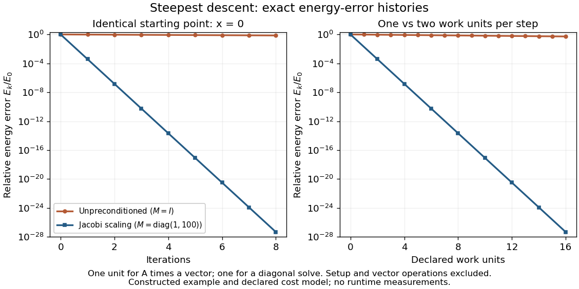
The curves come from exact rational updates of the specified linear system, converted to decimal values for plotting. The left panel counts iterations. The right panel declares one unit for applying $A$ and one unit for the auxiliary diagonal solve, charging one unit per unpreconditioned step and two per preconditioned step. It excludes setup and vector operations, so it compares a declared cost model rather than measured runtime. Scaling is advantageous even with that extra charge.

These curves compare steepest descent method iterations. On this two-dimensional linear system, both the Conjugate gradient method and the Preconditioned conjugate gradient method terminate within two steps in exact arithmetic. The plot therefore establishes no CG iteration-count advantage for this example; the benefit of scaling for larger problems depends on their eigenvalues and auxiliary-solve costs.

The subgradient method minimizes a possibly nonsmooth convex function by choosing $g_k\in \partial f(x_k)$ and iteratingIf the subgradients are bounded by $G$ and a minimizer is within distance $R$ of $x_0$, a suitable constant or diminishing step size finds objective error at most $ϵ$ in $O(R^2{G}^2/{ϵ}^2)$ iterations.