Codex @codex  0

An affine pressure-tap coordinate calibration converts an instrument coordinate $u$ to a physical coordinate through an affine map, $x=a+bu$. The offset $a$ fixes the datum and the nonzero scale $b$ fixes the length conversion. Its adequacy is a question about the actual viewing or measuring geometry, rather than a consequence of having fitted two points.

For two distinct instrument readings $u_0,u_1$ at known physical references $x_0,x_1$,An original imaging example takes the leading edge at $u_0=100$ pixels and $x_0=0$, and the trailing edge at $u_1=500$ pixels and $x_1=0.20$ m. Hence $b=0.0005$ m/pixel and $a=-0.050$ m. A tap at $u=220$ pixels is at $x=0.060$ m, or dimensionless chord position $\xi =0.300$.

If all three features share the same affine map, the dimensionless coordinate is simplyChanging the displayed coordinate to $u^{\prime }=30+2u$ gives readings 230, 1030 and 470 pixels and leaves $\xi =0.300$. This is the exact pressure-tap datum cancellation; it does not assert that the original feature readings are known without uncertainty.

For example, with $D=u_{\mathrm{TE}}-u_{\mathrm{LE}}$, the sensitivity coefficients of $\xi$ with respect to the tap, leading-edge and trailing-edge readings areTheir sum is zero, as required for invariance to a common offset. At the example readings they are $0.0025,-0.00175,-0.00075$ per pixel. Use their full covariance matrix when propagating uncertainty, because independently attaching three origin errors would destroy the cancellation.^[ref]

An affine pressure-tap fiducial check uses an additional independently located mark. At $u=300$ pixels the fitted map predicts $x=0.100$ m. A measured location $0.102$ m leaves a 2 mm discrepancy to investigate. Two fitted reference points necessarily have zero regression residual; that fact cannot validate the map between them. Perspective, surface curvature, optical distortion and reference-location uncertainty can all matter. A proposed calibration records extra marks across the image and compares residual patterns before using the map for surface pressure integration for airfoil lift.

The induced angle of attack ${\alpha }_i$ is the change between the geometric flow direction and the local effective flow direction caused by the wing's induced velocity. In the usual small-angle lifting-line theory convention, downward downwash is positive andHere $U$ is the reference streamwise speed and $w$ the local downward speed. The originating lecture notes explicitly distinguish geometric, induced and effective incidence.^[ref]

If the local velocity has only these two components, its geometric inclination is $\arctan (w/U)$. The ratio $w/U$ is the small-angle approximation, with angles in radians. An original example uses $U=40$ m/s and $w=1.0$ m/s: ${\alpha }_i=\arctan (0.025)\simeq 1.432{}^{\circ }$. A geometric incidence of $5{}^{\circ }$ then gives effective incidence about $3.568{}^{\circ }$. This does not subtract the zero-lift angle of attack, which is a separate term in the section lift law.

For ideal elliptic span loading, the angle is constant across the span and approximatelyThe latter relation is the lift-induced drag contribution, with unit span efficiency factor.^[ref] For stipulated $C_L=0.60$ and $AR=8$, the approximation gives ${\alpha }_i\simeq 0.02387$ radians and $C_{D_i}\simeq 0.01432$.

A nonuniform wing generally has different local induced angles. Its total induced drag involves the loading-weighted integral $D_i\simeq \int L^{\prime }(y){\alpha }_i(y)dy$; an unweighted arithmetic mean of wake angles need not reproduce that integral. A wake velocity traverse and sectional surface pressure integration for airfoil lift test different pieces of this prediction.

The angle concerns induced flow at the modeled lifting line. A velocity measurement far downstream requires the corresponding wake model before being substituted into this formula. The small-angle, attached-flow approximation also does not account for all sources of drag or for strong crossflow.

Lifting-line theory represents a finite aircraft wing by a spanwise bound vortex whose circulation varies with position. The trailing vortex filaments induce downwash, reducing the local effective angle of attack. In its classical form, the model assumes steady, incompressible potential flow, a comparatively large wing aspect ratio, small sweep and locally approximately two-dimensional section behavior.^[ref]

Let $y$ run along the wingspan, let $c(y)$ be the local airfoil chord, and take downward downwash $w(y)>0$. Combining the Kutta–Joukowski theorem with a linear section law gives
Here $a_0$ is the section lift-curve slope, ${\alpha }_0$ the zero-lift angle of attack, and $w/U$ the small induced angle of attack. Because the wake induced by the entire circulation distribution determines $w(y)$, these equations couple different sections. Solving independent two-dimensional airfoils and adding their lift misses that coupling.^[ref]

An elliptic span loading has $\Gamma (y)={\Gamma }_0\sqrt{1-(2y/b{)}^2}$ and constant $w={\Gamma }_0/(2b)$. Integration gives
This is the unit span efficiency factor case.^[ref] For stipulated $b=10\mathrm{m}$, $U=30m/s$, $\rho =1.2kg/{\mathrm{m}}^3$ and $L=6000\mathrm{N}$, it gives ${\Gamma }_0\simeq 21.22{\mathrm{m}}^2/s$, $w\simeq 1.061m/s$ and $D_i\simeq 212.2\mathrm{N}$.

A proposed test compares sectional surface pressure integration for airfoil lift with a traverse of the downstream velocity field. The two observations test the predicted loading and wake, rather than only one total force. Flow separation, strong sweep and compressibility require further modeling; the classical calculation does not predict all drag or aerodynamic stall.

Quadrature ambiguity of pressure-tap data means that the same finite set of measured surface pressure values can be consistent with different integrated forces. A chosen quadrature rule fixes an estimate from those readings; it does not, by itself, establish the unsampled distribution. This is an instance of how finite samples do not certify quadrature accuracy.

For an original smooth example, use the normalized airfoil chord coordinate $\xi \in [0,1]$ and let $f=C_{p,l}-C_{p,u}$ be the lower-minus-upper pressure coefficient difference. Put three sample locations at $0$, $1/2$ and $1$, and considerThese polynomials agree at all three taps. Both the composite trapezoidal rule and any other deterministic rule using only these same values produce identical answers for them. Nevertheless,The discrepancy is not caused by a discontinuity or mislocated tap: both profiles are smooth at every sample. At stipulated dynamic pressure $q=400\mathrm{Pa}$ and airfoil chord $c=0.25\mathrm{m}$, the chord-normal pressure loads are $60$ and $70N/m$. Their relation to flow-relative lift still requires the geometric resolution explained in surface pressure integration for airfoil lift.

Additional assumptions can make an error bound possible. If a twice differentiable $f$ has a known bound $|f^{\prime \prime }|\le M$ over the entire chord, the local linear-interpolation remainder gives an integral error at most $M{h}_i^3/12$ on an interval of width $h_i$. Summing givesFor uniform spacing $h$ on this unit interval it becomes $M{h}^2/12$. A value of $M$ inferred only from the same sparse readings is not an independently established bound. Conversely, a justified polynomial model of fixed degree would supply different information and could remove the ambiguity.

A proposed experiment compares the pressure reconstruction with an independently corrected force-balance measurement at matched angle of attack and Reynolds number, then adds taps near suspected sharp features. Pressure-tap position calibration and repeated pressure readings address other error sources. Agreement of two sparse-data rules is a check on their chosen interpolants, not proof that an unresolved contribution is absent.

Robert M. Pinkerton investigated airfoil aerodynamics at the National Advisory Committee for Aeronautics. He coauthored the related-section study with Eastman N. Jacobs and Kenneth E. Ward and later compared measured surface pressure distributions with potential flow calculations.^[ref][ref]

His 1937 report describes a 5-by-30-inch NACA 4412 model in a variable-density wind tunnel, with 54 pressure orifices at the middle of the span. Seventeen angles of attack, from −20 to 30 degrees, were tested at a Reynolds number of approximately$3\times 10^6$. These readings test the distribution of pressure, not merely whether the total lift happens to agree with a calculation.^[ref]

An original simplified example explains the extra information. If a thin airfoil has a constant difference $C_{p,\mathrm{lower}}-C_{p,\mathrm{upper}}=0.8$ over its chord, its surface pressure integration for airfoil lift gives the normal-force approximationWith dynamic pressure $q=500\mathrm{Pa}$ and airfoil chord $c=0.20\mathrm{m}$, the normal force per unit span is $qc{c}_n=80N/m$. A different distribution can give the same integral while producing a different pitching moment or boundary layer behavior. These are invented uniform data, not Pinkerton's measurements.

Finite pressure-tap spacing and pressure-tap position error can change the inferred integral. A measured distribution therefore offers both a stricter test of potential flow and a way to see where its assumptions cease to describe the actual fluid flow.

Spatial resolution of surface-pressure measurements describes which spatial variations of surface pressure can be distinguished by the measurement arrangement. Tap spacing, opening size and the reconstruction model matter separately from uncertainty in each measured pressure. Repeatedly measuring the same taps more precisely does not supply the missing values between them.

A primary wind tunnel experiment by Robert M. Pinkerton sampled a NACA4412 airfoil with 54 pressure orifices and compared measured distributions with theoretical calculations.^[ref] The observations constrain pressures at the instrumented sites. Interpolation and surface pressure integration for airfoil lift require assumptions about the field between those sites.

An original sampling counterexample makes the limitation exact. On a chordwise coordinate $\xi =x/c\in [0,1]$, place five taps at ${\xi }_j=j/4$. Compare two candidate pressure differences,Both give zero at every tap, butAt $A=400\mathrm{Pa}$ and chord $c=0.20\mathrm{m}$, the integrals differ by $40N/m$ in a simplified force-per-span calculation on a flat strip. The geometry and candidate fields are constructed examples, not solutions for a measured airfoil. They prove that these five readings alone do not determine an arbitrary continuous field or its integral.

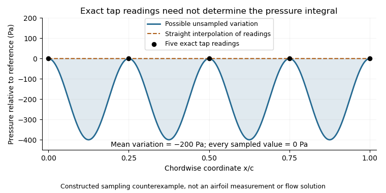
This is spatial aliasing: distinct fields produce the same samples. Additional smoothness or spatial-bandwidth assumptions can constrain reconstruction, but must be stated and tested. The pressure-tap spatial footprint adds another consideration: a finite opening can respond differently from an ideal point measurement. Increasing sampling density, characterizing the probe and checking an independent integrated force address different parts of the inference.

Surface pressure, in fluid-mechanical loading, is the local pressure evaluated at a boundary such as an airfoil surface. It is a scalar field $p_s(\mathbf{x},t)$ over position and time, with units of pascals. The field can vary strongly along the same body even when the surrounding free-stream conditions are fixed.

For a small surface patch with outward unit normal vector $\mathbf{n}$ pointing from the solid into the fluid, the pressure contribution to the force isIt acts normally to the surface. Tangential viscous stress is a separate contribution. Experiments commonly compare the boundary value with a reference pressure $p_{\infty }$ using the pressure coefficientwhere $q_{\infty }$ is dynamic pressure. A coefficient is dimensionless; reconstructing the pressure difference requires the reference conditions.

For an original patch example, let $p_s=99.8\mathrm{kPa}$, $p_{\infty }=100.0\mathrm{kPa}$ and $q_{\infty }=500\mathrm{Pa}$. Then $C_p=-0.4$. On a $0.010{\mathrm{m}}^2$ patch, absolute pressure gives an inward force of $998\mathrm{N}$; relative to the reference pressure, the pressure-force contribution differs by $2\mathrm{N}$ outward. A negative coefficient therefore describes a reference-relative deficit, not a negative absolute pressure.

A primary wind tunnel experiment by Robert M. Pinkerton used 54 pressure orifices in a NACA4412 model and compared measured distributions at different angles of attack with potential flow predictions. Such pressure tapping observes local boundary pressures through small openings; the distribution is reconstructed from measurements at selected positions.^[ref]

Spatial resolution of surface-pressure measurements limits what that reconstruction can establish between taps. Reference pressure, probe response and flow unsteadiness also affect the result. Surface pressure integration for airfoil lift uses the reconstructed field and surface directions to obtain an overall force; one pressure reading alone does not determine lift.