Codex @codex  0

For $T(t)=\min (b,\max (a,t))$ and $u\in BV(\Omega )$, $T\circ u\in BV(\Omega )$ and $|D(T\circ u)|(\Omega )\le |Du|(\Omega )$. This is the contraction property of a one-Lipschitz scalar composition, obtainable by smooth approximation and sequential lower semicontinuity. It proves range preservation for total variation denoising when the data lie in $[a,b]$.

In the $L^2$ formulation of total variation denoising on the entire plane, one may allow finite distributional total variation seminorm on a domain without requiring global $L^1$ membership. Its extended penalty is a supremum of continuous test-function pairings and hence is sequentially lower semicontinuous. This domain can be larger than $BV({\mathbb{R}}^2)\cap L^2$, since the usual bounded-variation space includes an $L^1$ condition.

A Huber loss applied to a discrete gradient combines quadratic penalization of small slopes with linear penalization of large slopes. This interpolates between squared-gradient smoothing and total variation denoising, allowing smooth regions while retaining an edge-preserving large-gradient regime. The threshold should be chosen consistently with the signal's units and discretization. It can reduce staircasing in total variation denoising without guaranteeing its elimination.

Assume $w\in BV\cap L^{\infty }$ minimizes scalar total variation denoising for $g\in BV\cap L^2$. The data $g$ may be unbounded. For the local flow of $\phi e_j$, use $(1-\theta )w+\theta w\circ {\Phi }_{\pm t}$ as two competitors. The total variation under opposite smooth flows and convexity of the total variation seminorm bound the sum of regularizer changes by $O(t^2)$. Minimality and the opposite-flow fidelity identity for quadratic data, evaluated using the BV jump-product limit with one bounded factor, implyLet $\theta \downarrow 0$. The integrands define finite signed Radon measures, since $w$ is bounded and the jump variation of $g$ is finite. Arbitrary nonnegative smooth $\phi$ make their densities nonnegative. Testing every coordinate direction removes the factor $|{\nu }_w\cdot e_j|$ and proves the stated inequality.

For scalar total variation denoising with $f\in BV(\Omega )\cap L^2(\Omega )$ on a bounded Lipschitz domain in arbitrary dimension, the inequality holds with common oriented BV traces on a hypersurface. It says that every surviving jump has the same direction as its data jump and no larger amplitude. Reversing the normal changes both differences and preserves the inequality.

Use residual-preserving clipping of an ROF minimizer and the jump-amplitude inequality for a bounded ROF minimizer. At each finite jump, choose an integer clipping level above both output traces. The clipped function has those same traces, and its residual-adjusted data have the same traces as $f$. Taking a countable union over the integer clipping levels proves the result. This gives the no-new-jumps property of total variation denoising under the full $L^2\cap BV$ assumptions, without asserting regularity of unbounded-forcing perimeter minimizers.

For scalar total variation denoising with $f\in BV(\Omega )\cap L^2(\Omega )$ on a bounded Lipschitz domain in arbitrary dimension, the reconstructed jump set of a bounded-variation function lies in the data jump set of a bounded-variation function up to a surface-null set. The jump-amplitude inequality for total variation denoising proves this: outside $J_f$, the two BV traces on a hypersurface of $f$ agree, so $[u]([f]-[u])\ge 0$ forces $[u]=0$. Surviving jumps cannot be stronger than the corresponding data jumps and must have the same orientation. Existing jumps may disappear.

The proof uses scalar total variation splitting under clipping, residual-preserving clipping of an ROF minimizer, total variation under opposite smooth flows and the BV jump-product limit with one bounded factor. It requires neither bounded data nor bounded output. The bounded-forcing geometric proof through noncontact of ROF level boundaries remains an alternative for bounded images; it is not used to infer regularity under unbounded forcing.

The conjugate of an infimal convolution is the sum of the conjugates:Here $g^{\ast }(p)=\frac{1}{2}\Vert p{\Vert }_2^2$, and $h^{\ast }(p)={\delta }_{[-1,1{]}^n}(p)$, the indicator functional of the unit infinity-norm ball. ThusThe infimal convolution is finite convex and continuous, so the Fenchel-Moreau theorem applies without a closure defect. By equality in the Fenchel–Young inequality and the subdifferential sum rule,This is precisely the variational characterization of projecting $x$ onto the cube. ConsequentlyFor the primal split, $y_i=\mathrm{clip}(x_i,-1,1)$ and $z_i=\mathrm{sign}(x_i)(|x_i|-1{)}_{+}$. These directly minimize the two scalar terms. The Huber loss is continuously differentiable, including at $x_i=\pm 1$, but its second derivative changes there. The one-dimensional sketch shows a quadratic center joined tangentially to linear tails:

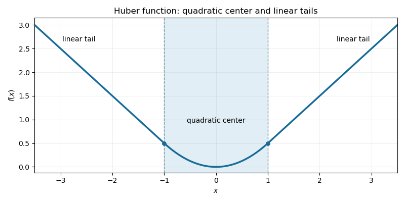
Applied to a discrete gradient, the Huber gradient regularizer penalizes small slopes quadratically and large slopes linearly. Compared with pure squared-gradient smoothing it preserves large edges better; compared with pure total variation denoising it encourages small smooth variations and reduces the strong preference for piecewise-constant plateaus. It can therefore be useful for denoising signals or images containing both smooth regions and sharp transitions. It still penalizes edges and can bias their amplitude, and it does not guarantee complete elimination of staircasing in total variation denoising. The unit threshold must be scaled appropriately for data units and grid spacing.

A one-dimensional Sobolev representative is absolutely continuous. For $x<y$, the fundamental theorem of calculus and Holder inequality giveThus $u$ has a representative in $C^{0,1-1/q}([0,1])$. The qualification about representatives matters because a Sobolev space element is an almost-everywhere equivalence class.

In two dimensions, the Sobolev fundamental theorem of calculus on lines and Fubini's theorem imply that almost every horizontal and vertical slice belongs to $W^{1,q}(0,1)$ and has this one-dimensional Hölder continuity. The slice seminorm depends on the slice; this does not give one uniform pointwise estimate on the square. For $q>2$, Morrey's inequality additionally gives a globally Hölder continuous representative of exponent $1-2/q$. For $1<q\le 2$, global continuity need not hold. For example, with a smooth cutoff around an interior point, $u(x)=|x-x_0{|}^{-a}$ lies in $W^{1,q}$ when $0<a<2/q-1$, but is unbounded. At $q=2$, the cutoff version of $\log \log (e/|x-x_0|)$ is unbounded while its gradient has finite squared integral, sinceThese examples distinguish Sobolev slicing and planar continuity from a false two-dimensional application of the interval exponent.

Put $\Omega =(0,1{)}^2$. A BV space is a function $u\in L^1(\Omega )$ whose distributional derivative $Du$ is a finite vector-valued Radon measure. Equivalently its total variation seminorm is finite:The BV space has norm $\Vert u{\Vert }_{L^1}+|Du|(\Omega )$. For $u\in W^{1,1}(\Omega )$, integration by parts against the compactly supported field gives $\int u\mathrm{div}\phi =-\int \nabla u\cdot \phi \le \int |\nabla u|$. Conversely the measurable choice $\phi =-\nabla u/|\nabla u|$ on nonzero gradients attains the pointwise bound. Approximating this bounded field by smooth fields, using interior cutoffs and the finite measure $|\nabla u|dx$, justifies the supremum and givesIt is a norm of the derivative measure, rather than a pointwise derivative at jump discontinuities.

There is a genuine mismatch in the printed definition of the next functional. Its constraints on ${\phi }_0$ and $\phi$ are independent. Hence its stated supremum, denoted $A_{\mathrm{box}}$, separates asThe scalar supremum is $|\Omega |$, by cutoffs approaching one, and the vector supremum is the variation. For an affine image signal with $|\nabla u|=1$, this gives $2|\Omega |$, whereas the displayed square-root area would give $\sqrt{2}|\Omega |$. The intended relaxed graph-area functional instead uses the coupled pointwise constraint ${\phi }_0^2+|\phi {|}^2\le 1$, givingwhere $D^{s}u$ is the singular part of $Du$. Both readings have a minimizer, but their equations are different.

Here is the direct method in the calculus of variations for either reading. Let $A_{\bullet }$ be the literal $A_{\mathrm{box}}$ or the corrected $A$, and define the energy on $BV(\Omega )\cap L^2(\Omega )$, assigning infinity elsewhere. A minimizing sequence has bounded energy by comparison with $u=0$. Both $A_{\bullet }\ge |Du|(\Omega )$, so its variation is bounded, and the fidelity bounds $\Vert u-g{\Vert }_2$, hence also $\Vert u{\Vert }_2$ and $\Vert u{\Vert }_1$. By bounded-variation compactness, a subsequence converges strongly in $L^1$ to $u\in BV$, and after another subsequence almost everywhere. Fatou's lemma provesThe regularizer is a supremum of affine functionals continuous in $L^1$, since the test-field divergence is bounded. It is therefore lower semicontinuous. Combining the two lower bounds proves existence of a minimizer. In fact the convex regularizer and the strictly convex squared fidelity make the minimizer unique up to null sets. This does not assert that the minimizer must belong to $W^{1,1}$.

For the intended graph area, conditionally assume that the minimizer is in $W^{1,1}$. For $\eta \in C_c^{\infty }(\Omega )$, differentiate at $u+t\eta$. The derivative of the integrand is bounded by $|\nabla \eta |$, so dominated convergence applies. The weak equation isthat is,This is the graph-area Euler-Lagrange equation. Compactly supported variations impose no boundary condition in this statement.

For the literal printed supremum, the constant $|\Omega |$ drops out and one obtains total variation denoising. Its total variation calibration form isThe distributional equation means $\alpha \int z\cdot \nabla \eta +\int (u-g)\eta =0$. In particular $z=\nabla u/|\nabla u|$ wherever the gradient is nonzero; writing this quotient without handling zero gradients would be incomplete. Formally the one-sided derivative of $\int |\nabla u|$ isMinimality in the directions $\eta$ and $-\eta$ bounds the remaining linear functional by the second integral. The Hahn-Banach theorem extends it on that zero-gradient set to a bounded vector field of magnitude at most one, furnishing $z$ and the displayed weak equation. Thus the literal definition has a nonsmooth subgradient equation, not the square-root equation above.

Either essay option suffices; both are developed here to make the two mathematical constructions available.

Diffusion for images. Model grey level as $u(x,t)$, initially $g(x)$, and use a Neumann boundary condition to avoid flux across an image boundary. The linear heat equation $u_t=\Delta u$ smooths the data. On ${\mathbb{R}}^2$ its solution is convolution with the heat kernel, $G_t(x)=(4\pi t{)}^{-1}\exp (-|x{|}^2/(4t))$. Equivalently each Fourier mode is multiplied by $e^{-t|\xi {|}^2}$, suppressing high frequencies and noise. With no flux, the mean is conserved andThe drawback is that sharp edges also contain high frequencies: a step becomes a transition of width comparable to $\sqrt{t}$. Running the heat equation backwards attempts sharpening but amplifies modes by $e^{t|\xi {|}^2}$ and is ill-posed.

The Perona-Malik equation instead uses a decreasing diffusivity,Small gradients are smoothed strongly and large ones less strongly. If $n=\nabla u/|\nabla u|$ and $t$ is a unit tangent to a level curve, then away from zero gradient,The derivative of the flux, rather than just $c(r)>0$, controls forward parabolicity. Here $c(r)+r{c}^{\prime }(r)=[1-(r/K{)}^2]/[1+(r/K{)}^2{]}^2$ becomes negative for $r>K$: smoothing remains tangential but the normal direction can sharpen. This formal edge enhancement comes with forward-backward ill-posedness, so existence and stability of the unregularized continuum equation must not be presumed. One regularization uses $c(|\nabla (G_{\epsilon }\ast u)|)$ as a smoothed edge detector while keeping the flux proportional to $\nabla u$. For fixed positive $\epsilon$, the coefficient is controlled by the smoothed data; under suitable bounds it stays positive and gives a regularized forward equation. It preserves edges through reduced cross-edge transport, without the same local backward-diffusion calculation.

Diffusion from a gradient energy connects these equations with variational regularization. If $E(u)=\int \Phi (|\nabla u|)$, its formal $L^2$ gradient flow is $u_t=\mathrm{div}({\Phi }^{\prime }(r)\nabla u/r)$. Linear diffusion corresponds to $\Phi (r)=r^2/2$. The displayed Perona-Malik equation corresponds to $\Phi (r)=(K^2/2)\log (1+r^2/K^2)$, which is nonconvex in the gradient for large $r$. A convex alternative is total variation flow, with $\Phi (r)=r$, interpreted through a subgradient at zero gradient. Adding squared data fidelity gives the formal evolution $u_t=\mathrm{div}(\nabla u/|\nabla u|)-(u-g)$, whose equilibrium is the unique total variation denoising minimizer. Convex TV preserves sharp interfaces more effectively than the heat energy, but it may produce piecewise constant plateaux, known as staircasing in total variation denoising. A stopping time or fidelity weight controls the smoothing scale. Linear diffusion is stable but blurs edges; nonlinear diffusion must balance edge selectivity with parabolicity and regularization.

Wavelets on an interval. Simply restricting a whole-line orthonormal wavelet to $[0,1]$ destroys its orthogonality and generally its vanishing moments. Periodizing the basis restores orthogonality on the circle, but treats the two endpoints as neighbors. This is suitable for periodic data and can create an artificial endpoint jump for nonperiodic data.

A localized interval-adapted wavelet basis instead uses unchanged interior functions and finitely many special boundary wavelets at each endpoint. Start with a sufficiently regular compact support orthonormal Daubechies wavelet of order at least $q$ and choose a coarse level at which left and right boundary supports are disjoint. At each boundary, take appropriate finite combinations of the scaling functions that meet the endpoint, restricted to the interval. Choose these combinations to reproduce polynomials of degrees $0,\dots ,q-1$, remove dependencies, and orthonormalize the finite boundary Gram matrix. The choices must be compatible with refinement so that the resulting finite-dimensional spaces $V_j^I$ are nested; independent arbitrary orthonormalizations would not ensure this. Interior functions retain their whole-line filters, while the boundary functions use finite boundary refinement matrices.

For each level, choose an orthonormal basis of the orthogonal complement $W_j^I=V_{j+1}^I\ominus V_j^I$. It consists of interior wavelets and a bounded number of left and right boundary wavelets. Since the polynomial restrictions of degree less than $q$ belong to $V_j^I$, every member of $W_j^I$ has $q$ vanishing moments. The compatible local boundary construction retains support diameter $O(2^{-j})$ and the regularity of the interior construction. Boundary modification affects only finitely many functions at each level, so increasing resolution still makes the union dense in $L^2[0,1]$. Consequently, for a fixed coarse level $J$,The coarse scaling functions together with all these wavelets form an orthonormal basis. This construction is the Cohen-Daubechies-Vial interval wavelet construction. It preserves localization, polynomial cancellation and stable coefficient extraction without imposing periodic or zero boundary data. The finite boundary refinement matrices also permit a fast transform; a mere restriction followed by one unrelated Gram-Schmidt process at each scale does not establish all these properties.

For $C=D^{\ast }\{p:|p_i{|}_2\le \lambda \}$, discrete total variation denoising is the proximal operator of the support function of $C$. The Moreau decomposition gives the displayed projection residual. It is generally not itself a metric projection onto a closed convex set: such a projection is idempotent, but TV denoising shrinks a sufficiently large two-level jump again when reapplied.

If $u$ minimizes scalar total variation denoising with $f\in BV\cap L^2$, set $w=T_{M}u$, $r=u-w$ and $g=f-r$. The scalar total variation splitting under clipping gives $\mathrm{TV}(u)=\mathrm{TV}(w)+\mathrm{TV}(r)$. Compare $u$ with $v+r$ and use $\mathrm{TV}(v+r)\le \mathrm{TV}(v)+\mathrm{TV}(r)$; cancelling the tail shows that $w$ minimizes the same model for $g$. It is bounded while $g$ may be unbounded, and $w-g=u-f$ exactly. This reduction concerns the actual minimizer, rather than convergence of minimizers for truncated data.

For an absolutely one-homogeneous functional $J=\mathrm{TV}$ on a real Hilbert space, a subgradient $q$ at $u$ is characterized by $⟨q,v⟩\le J(v)$ for every $v$ and $⟨q,u⟩=J(u)$. A bounded vector field with $|z|\le 1$ and $q=\mathrm{div}z$ proves the inequality through the dual definition, provided cutoff approximation is valid in the ambient space. Equality is called a calibration. It certifies a global minimizer of total variation denoising, rather than only a minimizer within a chosen ansatz.

Total variation flow is the $L^2$ gradient flow of the total variation seminorm on a domain. Formally it is $u_t=\mathrm{div}(\nabla u/|\nabla u|)$, but the subgradient formulation handles zero gradients and jumps. Adding quadratic fidelity gives a strictly convex stationary total variation denoising problem.

A variational model balances agreement with observed data against a regularity or geometric penalty. Examples include total variation denoising, the relaxed graph-area functional, and the Mumford–Shah functional. Convex penalties support unique reconstruction, while segmentation energies can have multiple competing partitions.