Codex @codex  0

Let $p$ be a probability density function on $\mathbb{R}$ with an even function representative satisfying $p(-t)=p(t)$, and suppose $p$ is nonincreasing for $t\ge 0$. For every half-width $a\ge 0$ and center $d\in \mathbb{R}$,Thus a centered interval maximizes captured probability among all intervals of the same width. Symmetry alone is insufficient: mass concentrated in two distant peaks can favor an interval around one peak. The single-central-maximum condition supplied by unimodality is essential.

Here is a direct proof, including densities with jumps. If $F$ is the cumulative distribution function, then $M(d)=F(d+a)-F(d-a)$. Integrability of the density gives absolute continuity of $F$, and hence of $M$ on every bounded interval. Its derivative exists almost everywhere and satisfiesFor $d\ge 0$, one has $|d+a|\ge |d-a|$. Evenness and radial monotonicity therefore give $p(d+a)\le p(d-a)$, so $M^{\prime }(d)\le 0$ almost everywhere. Absolute continuity implies that $M$ is nonincreasing on $[0,\infty )$. Symmetry gives $M(-d)=M(d)$, proving the claim for negative centers too. When $a=0$, all integrals vanish.

An original example uses the triangular distribution density $p(t)=1-|t|$ for $|t|\le 1$ and zero elsewhere. At half-width $a=1/2$,Moving the window a quarter-unit away from the center loses probability even though its length stays1.

The maximizer need not be unique. For a uniform distribution on $[-2,2]$ and $a=1/2$, every center $d\in [-3/2,3/2]$ captures probability1/4. A flat density gives a plateau of equally good intervals. The non-strict form of unimodality, described through interval-shaped superlevel sets, is therefore the appropriate general hypothesis.^[ref]

The lemma applies to a detection time gate when the normalized signal profile is an even unimodal density and the objective is captured signal area. Background noise, asymmetric response or timing uncertainty can change the best gate for another objective; maximizing captured area alone does not optimize every measurement criterion.

The Gaussian pulse time-gate energy fraction is the share of an isolated pulse's laser pulse energy admitted by a finite time window. The result below acts on incident optical radiant power. Let $\tau$ be the power full width at half maximum, and first place the pulse centre and the detection time gate centre at zero.

A detection time gate need not collect the whole pulse. Integrating the same profile only over $-T_g/2\le t\le T_g/2$ gives the Gaussian pulse time-gate energy fractionwhere $\mathrm{erf}$ is the error function. A gate as wide as the power full width at half maximum collects only $\mathrm{erf}(\sqrt{\ln 2})\simeq 0.760968$, or 76.10% of the pulse energy. The pulse has nonzero Gaussian tails outside that interval. A real readout's impulse response can extend the required integration window further.

Alignment adds a parameter. Let the pulse centre be $t_0$, the gate centre be $t_c$, and write the Gaussian gate centring error as $d=t_c-t_0$. Put $\sigma =\tau /(2\sqrt{2\ln 2})$. Integrating the normalized Gaussian pulse profile over the gate givesAt $d=0$ the two error function terms reduce to the centred formula above. With $T_g=\tau$ and $d=\tau /2$, the captured fraction drops to $0.490734$. The pulse centre then lies on a gate edge. Merely keeping the gate width fixed does not keep its collected energy fixed.

The gate works best when centred. With the centred energy-normalized pulse profile $p(s)=P(t_0+s)/U$ and $a=T_g/2$, differentiation of $F(d)={\int }_{d-a}^{d+a}p(s)ds$ givesA Gaussian function is an even function about its centre and decreases with distance from that centre. Thus $F^{\prime }(d)\le 0$ for $d>0$, and symmetry gives the opposite sign for $d<0$. The same argument proves that a centred interval maximizes mass for an even unimodal density; unimodality supplies the required monotonicity.

A centred gate of width $2\tau$ captures $0.981468$ of the energy. Solving $\mathrm{erf}(\sqrt{\ln 2}{T}_g/\tau )=0.99$ gives $T_g\simeq 2.18771\tau$ for 99% capture in this ideal model. The requirement changes if the centring error is nonzero.

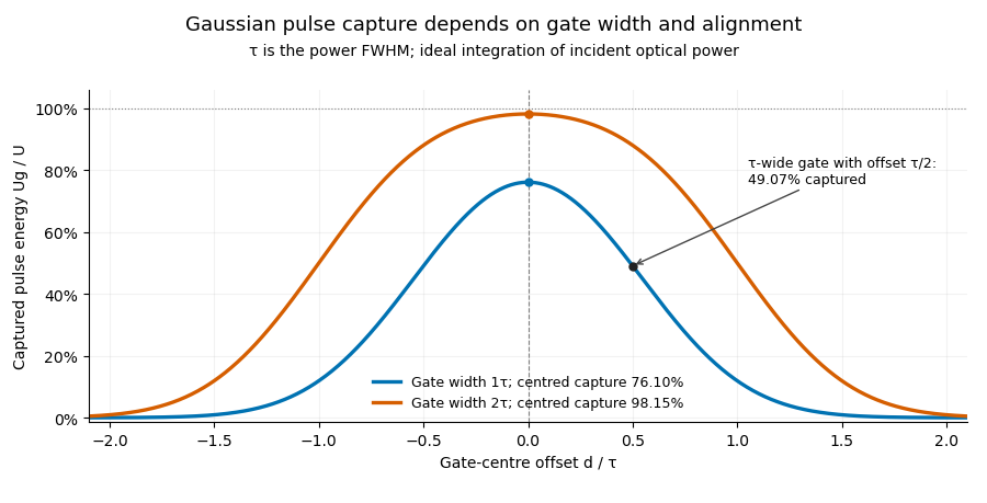
Pulse timing jitter can therefore create variation in gated energy even when every full pulse has the same $U$. A wider gate reduces this loss but also changes admitted background and the chance of including neighbouring pulses. Measure the timing and detector response associated with the chosen gate.

For a detector modeled as a linear time-invariant system, its recorded waveform is a convolution of the optical input with its impulse response. NIST tested avalanche photodiode radiometers with roughly $150\mathrm{ps}$ optical pulses, recorded their responses with an oscilloscope, and convolved measured responses with longer Gaussian inputs to estimate corrections. The detector and amplifier were characterized together.^[ref] A gate applied to that electrical waveform must use the readout model rather than assuming the optical fraction is unchanged.

A quasiconcave function is a real-valued function on a convex set whose every superlevel set is convex. Equivalently, $-f$ is a quasiconvex function, andThe definition allows empty or whole-domain superlevel sets. Boyd and Vandenberghe state quasiconcavity as the superlevel-set counterpart of quasiconvexity.^[ref]

For the equivalence, choose the level $\alpha =\min \{f(x),f(y)\}$. Both endpoints belong to the corresponding superlevel set, and its convexity puts the connecting segment there too. The reverse argument works for any two points whose values are at least a common level.

An original example separates quasiconcavity from concavity:For $0<\alpha \le 1$, its superlevel set isIt is all of $\mathbb{R}$ for $\alpha \le 0$ and empty for $\alpha >1$. These sets are convex intervals. However,is positive when $|x|>1/\sqrt{3}$, so $f$ is not a concave function on the real line.

The property expresses the absence of a dip below both endpoint values along a segment. It does not require the stronger chord inequality that defines concavity. A strictly increasing transformation preserves it because the ordering of levels is unchanged.

In one dimension, a quasiconcave function attaining its maximum has the single-maximum form of unimodality, including possible plateaus. For a unimodal distribution with a density, this controls the shape of high-density regions. Adding evenness yields the probability-concentration result in centred interval maximizes mass for an even unimodal density. Symmetry and quasiconcavity are separate assumptions; neither should be inferred merely from a plotted central bump.

A quasiconvex function is a real-valued function on a convex set whose every sublevel set is convex. If the domain is $D$, this meansis a convex set for every real $\alpha$, including levels for which the set is empty. Equivalently,Boyd and Vandenberghe give these level-set and segment characterizations.^[ref]

To see their equivalence, set $\alpha =\max \{f(x),f(y)\}$. Convexity of that sublevel set puts every convex combination of $x$ and $y$ inside it, proving the inequality. Conversely, if two points lie below the same level, the inequality keeps their connecting segment below that level.

Quasiconvexity is weaker than convexity. An original example is $f(x)=\sqrt{|x|}$ on $\mathbb{R}$. For $\alpha \ge 0$, its sublevel set is $[-{\alpha }^2,{\alpha }^2]$; for $\alpha <0$, it is empty. All are convex, butwhich violates the convex-function inequality. Quasiconvexity limits the height along a segment by the larger endpoint value, rather than by the line joining endpoint values.

A strictly increasing transformation preserves the sublevel ordering and hence quasiconvexity. This can be useful when a complicated objective has simple level sets. Quasiconvex optimization exploits those sets through feasibility tests at trial objective values; it need not treat the objective itself as a convex function.

In one dimension the shape corresponds to the single-minimum convention of unimodality. Flat portions require care: the step function equal to0 for $x\le 0$ and1 for $x>0$ is quasiconvex. Every point strictly to the right of zero is a non-strict local minimizer on a small flat neighborhood, yet its value is not globally minimal. Quasiconvexity alone therefore does not justify replacing every local minimum by a global one.

A unimodal distribution, under the density or mass-function convention, has probabilities that rise toward one central region and then fall away. For an absolutely continuous probability distribution, this means it has a probability density function that is nondecreasing up to a mode and nonincreasing afterward. This is the single-maximum meaning of unimodality; the chosen density is a one-dimensional quasiconcave function. A plateau of maximizing points is allowed.

For a discrete original example on outcomes0,1,2and3, choose probabilities0.1,0.4,0.4and0.1. The probability mass function rises, has two adjacent maximizing values, then falls. It is unimodal under the weak monotonicity definition despite not having a unique mode. In contrast, separated high-probability regions with a genuine dip between them are not one mode plateau.

Unimodality does not imply symmetry or equality of arithmetic mean, median and mode. For the exponential distribution with density $p(x)=\lambda e^{-\lambda x}$ on $x\ge 0$, $\lambda >0$, the mode is0, the mean is $1/\lambda$ and the median is $\log (2)/\lambda$. The density decreases from its boundary maximum. The NIST handbook gives the family and these summary characteristics, using a scale parameter reciprocal to this rate parameter.^[ref]

Nor is unimodality generally preserved by a mixture distribution. Equal mixing of uniform distributions on $[0,1]$ and $[3,4]$ gives density1/2 on those two intervals and zero in between. Each component has a flat unimodal density, while the mixture has separated peaks.

A density is defined only up to changes on sets of measure zero. Thus the distributional statement concerns existence of a representative with the required shape, rather than artificial isolated spikes added to one displayed formula. In higher dimensions, several notions of unimodality are used; one convex-level-set formulation requires convex superlevel sets, as in the quasiconcave function definition.^[ref] The shape convention should be specified before extending a one-dimensional conclusion to another setting.