Laser pulse energy ($U=\int P(t)dt$)

Laser pulse energy is the radiant energy carried by one specified laser pulse across a measurement plane. For an isolated pulse whose total radiant power is $P(t)\ge 0$ and whose background is zero,Here $P$ is already integrated over the transverse beam area; it is not local irradiance. The unit of $U$ is the joule. Radiant exposure instead divides received energy by a receiving area, so a beam's $U$ alone does not specify the exposure at its centre. The radiant exposure of a Gaussian beam makes that spatial distinction quantitative.

The Gaussian pulse energy and peak power relation gives $P_{\mathrm{pk}}\simeq 0.939437U/\tau$ when $\tau$ is the power full width at half maximum. The pulse energy shape factor records pulse-shape dependence, while the Gaussian pulse field-envelope width is $\sqrt{2}$ times the power width.

For an original example, stipulate $U=0.50\mu \mathrm{J}$ and a Gaussian pulse power full width at half maximum $\tau =10\mathrm{ns}$. Then $P_{\mathrm{pk}}=46.97\mathrm{W}$. Stretching the same model pulse to $40\mathrm{ns}$ while keeping $U$ unchanged reduces its peak power to $11.74\mathrm{W}$. Both curves below integrate to the same energy; their peak heights and widths differ.

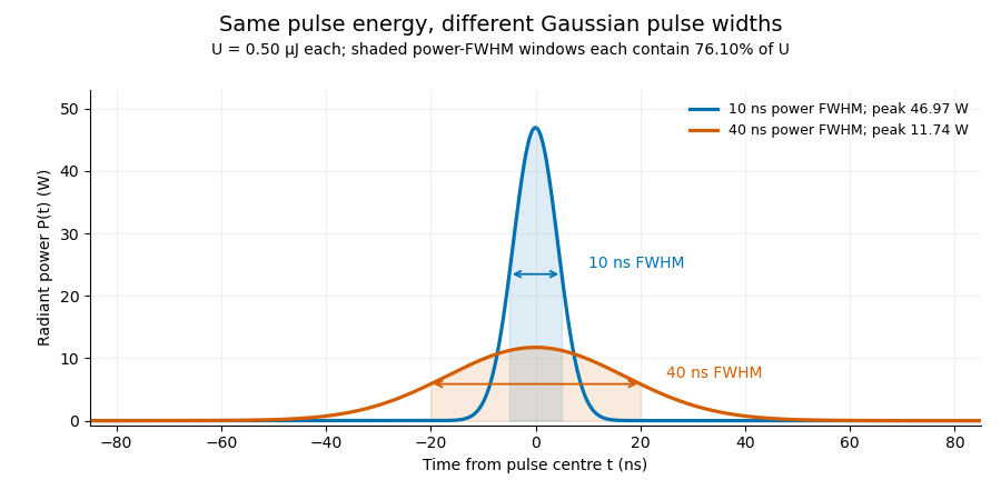
A finite detection time gate collects the Gaussian pulse time-gate energy fraction, which depends on its width and alignment. A centred gate as wide as the power full width at half maximum receives only $76.10\%$ of $U$, because Gaussian tails extend beyond it. For a $\tau$-wide gate, a Gaussian gate centring error of $\tau /2$ reduces capture to $49.07\%$.

The average power of a laser pulse train follows by counting complete pulses. If a long observation of duration $T$ contains $N$ pulses of energies $U_1,\dots ,U_N$, with negligible edge contributions and no continuous background,Here $f_{\mathrm{rep}}$ is the pulse repetition frequency, not the inverse pulse width. An average power readout constrains $\overline{U}$ when $f_{\mathrm{rep}}$ is known; it does not resolve pulse-to-pulse energy fluctuation. Identical, well-separated $0.50\mu \mathrm{J}$ pulses at $1.0\mathrm{MHz}$ give $0.50\mathrm{W}$ average power, even though the stipulated $10\mathrm{ns}$ pulses peak near $47\mathrm{W}$.

If a steady optical background is present, state whether the reported energy includes it. For pulse energy above a measured background $P_{\mathrm{bg}}$, the pulse energy baseline correction uses ${\int }_{\mathrm{gate}}[P(t)-P_{\mathrm{bg}}]dt$. Failing to subtract a constant background adds $P_{\mathrm{bg}}{T}_g$ to the inferred energy. This optical-background model is distinct from an offset introduced later by detector electronics.

Historical NIST equipment illustrates what the readouts measure. Its TC-24 reference absorbed the beam in a glass plate, sensed a plate temperature difference with thermocouples, and integrated the thermopile's electric potential difference during beam injection. Before/after readings enabled background subtraction and compensated thermal drift. Counting pulses converted total injected energy to mean pulse energy. The semiconductor pulse photodetector used an integrating amplifier; calibration related the peak output electric potential difference to pulse energy. That electrical peak did not by itself establish optical peak power.^[ref] Pulse energy measurement with a photodiode connects this kind of measurement to collected electric charge; validating the detector response under the actual pulse conditions remains part of that interpretation.