Codex @codex  0

The Conway polynomial is normalized by ${\nabla }_U=1$ for the unknot, zero for a split unlink with more than one component, and the skein relation ${\nabla }_{L_{+}}-{\nabla }_{L_{-}}=z{\nabla }_{L_0}$. For a knot, the symmetric Alexander polynomial with value one at $t=1$ is ${\Delta }_K(t)={\nabla }_K(t^{1/2}-t^{-1/2})$. This fixes the Laurent-unit ambiguity of the Seifert-matrix presentation of the Alexander module.

The Hopf link consists of two unknots with linking number $\pm 1$. Each component is a meridian of a knot of the other.

Resolve the two crossings in a skein relation using the Kauffman bracket, then correct by the writhe of a link diagram. The other smoothing cancels, leaving the displayed coefficient of the oriented smoothing. This relation and the value one on the unknot determine the Jones polynomial: crossing changes give descending diagrams, which are unlinks, while the smoothing terms have fewer crossings.

This asks whether the Jones polynomial equal to one characterizes the unknot among knots. A zero breadth of a Laurent polynomial makes $V_K$ a monomial; the identities $V_K(1)=1$ and $V_K^{\prime }(1)=0$ then force that monomial to be one. Thus using Jones breadth as a strictly positive complexity for nontrivial knots requires this detection property. To prove the derivative identity, differentiate the Jones polynomial skein relation at one for a crossing change in a knot. Both crossed diagrams have value one, while the smoothed two-component link has value minus two by Jones polynomial evaluation at one, so $V_{K_{+}}^{\prime }(1)=V_{K_{-}}^{\prime }(1)$. Crossing changes reduce to the unknot, whose derivative is zero. The corresponding Alexander polynomial detection property is false, as nontrivial untwisted Whitehead doubles demonstrate. The Jones question is discussed in research on closed four-strand braids.

A knot is the image $K=f(S^1)$ of a smooth embedding $f:S^1\hookrightarrow {\mathbb{R}}^3$, considered up to ambient isotopy. The circle $S^1$ supplies a closed loop with no free ends; the smooth embedding condition rules out self-intersections and requires a nonzero tangent vector in a regular parametrization. The equivalent convention $S^1\hookrightarrow S^3$ uses the three-sphere: removing a point outside the knot identifies the remaining space with three-dimensional Euclidean space by stereographic projection.

More precisely, knots $K_0,K_1$ are equivalent if there is a smooth family of diffeomorphisms $F_s$ of the ambient space, for $0\le s\le 1$, such that $F_0$ is the identity and $F_1(K_0)=K_1$. Every intermediate $F_s(K_0)$ remains a smooth embedding. This ambient isotopy allows bending, stretching and moving a loop, but neither cutting it nor letting strands cross through each other. We compare the embedded images rather than their parametrizations; an oriented knot additionally remembers a direction of travel.

For a worked example, start with $U(t)=(\cos t,\sin t,0)$, where $t$ is taken modulo $2\pi$, and useBoth scale factors stay positive, so each $F_s$ is a diffeomorphism. At $s=1$ the circle becomes the ellipse $(2\cos t,\frac{1}{2}\sin t,0)$, yet its knot type is still the unknot. Exact lengths and angles are therefore irrelevant to knot type; self-intersection is the obstruction that the deformation must avoid.

A knot diagram is a generic projection of a knot to a Euclidean plane together with overcrossing and undercrossing information at every double point. Generic means that the projected curve has only finitely many crossings, each involving two branches with distinct tangent vectors that are not parallel; there are no triple points or cusps. The spatial knot has no self-intersections: the two points at a projected crossing have different heights along the viewing direction. A gap in the lower strand records which one passes underneath.

Forgetting the over/under information leaves a knot shadow. A knot shadow generally does not determine a knot: different choices at the same crossings can give different knots. Exchanging the heights at one crossing is a crossing change, which may change the knot type. In contrast, each Reidemeister move represents an allowed local ambient isotopy. Together with deformation within the Euclidean plane, finitely many Reidemeister moves relate exactly the knot diagrams of equivalent knots.

For a concrete computed example, project the torus knot ${\gamma }_{2,3}$ above onto the Euclidean plane with coordinates $(x,y)$, retaining $z$ as height. Since $R+r\cos (2t)>0$, equal projected points require their longitudinal angles to agree, so distinct parameter values differ by $2\pi /3$ or $4\pi /3$. Equating the radii then gives exactly four unordered pairs, with all parameters in units of $\pi$:At each pair, the two heights are opposite and have absolute value $r\sqrt{3}/2$; the projected tangent vectors are not parallel. Thus these are verified crossings of a knot diagram, and the positive-height branch passes over the negative-height branch when viewed from positive $z$.

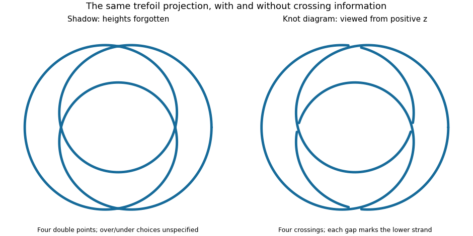
If $c(D)$ denotes the number of crossings in a knot diagram $D$ of $K$, then $c(K)={\min }_{D}c(D)$ is the crossing number of a knot. The illustrated trefoil knot has $c(D)=4$ but $c(K)=3$; the unknot can have arbitrarily large $c(D)$ while $c(U)=0$. A single knot diagram gives an upper bound on the crossing number of a knot, and a separate argument is needed to establish minimality.

Knot theory studies closed curves in three-dimensional Euclidean space that cannot intersect themselves, and asks which can be deformed into one another without cutting or passing one strand through another. Its basic object is a knot: a smooth embedding of a circle, considered up to ambient isotopy. Several disjoint knots form a link. More generally, knot theory studies such embeddings in other manifolds and in higher dimensions.

The central surprise is that a flexible circle can carry permanent information about how it sits in space. A trefoil knot and an unknot each consist of just one circle, but no ambient isotopy turns one into the other. A knot diagram translates this spatial question into a finite drawing; Reidemeister moves describe the changes of drawing that preserve the knot. Knot invariants translate it into computations: unequal Alexander polynomials of a knot, Jones polynomials, or knot groups certify different knots. Equal values of a particular knot invariant generally leave the question open; even an isomorphism of knot groups alone is not a complete classification.

An early foundation for working with knot diagrams is Kurt Reidemeister's 1927 paper Elementare Begründung der Knotentheorie, published in volume 5 of Abhandlungen aus dem Mathematischen Seminar der Universität Hamburg, pages 24–32.^[ref] Marc Lackenby's authored notes Elementary knot theory, Section 2.4, explain the Reidemeister move theorem and its role in searching for a certificate that two knot diagrams represent the same knot.^[ref]

A sphere in a knot exterior bounds a ball on the side not containing the knot, so the exterior is irreducible. A compression disk for its boundary torus would cut the exterior to a manifold with sphere boundary; irreducibility makes that manifold a ball, and reversing the compression gives a solid torus exterior. Its meridian disk has boundary a preferred knot longitude, so adjoining the boundary annulus gives a spanning disk for the knot, which is then an unknot. The Loop theorem therefore makes the peripheral fundamental group injective for every nontrivial knot. In particular its knot group contains an injected copy of the torus group and cannot be cyclic.

True with the stated Conway normalization. Fix $t^{1/2}=i$ at $t=-1$. The Jones polynomial skein relation becomesThe Conway polynomial satisfies ${\nabla }_{L_{+}}(z)-{\nabla }_{L_{-}}(z)=z{\nabla }_{L_0}(z)$. Put $W_L=(-1{)}^{\ell (L)-1}{\nabla }_L(2i)$. An oriented smoothing changes the number of components by one, so these quantities satisfy precisely $W_{L_{+}}-W_{L_{-}}=-2i{W}_{L_0}$. Both $W$ and $V(-1)$ are one on the unknot and zero on every multi-component unlink: for $V$, the split-union factor vanishes at this substitution.

These skein relations and unlink values determine the invariants uniquely. Switching a first undesired crossing gives a diagram closer to a descending diagram, while the smoothing term has fewer crossings; induction first on crossing count and then on undesired crossings reduces everything to unlinks. Thus $W_L=V_L(-1)$. For a knot there is one component and the Conway-normalized Alexander polynomial givesThis is the signed Jones evaluation at minus one. Replacing ${\Delta }_K$ by an arbitrary Laurent unit multiple would destroy the signed conclusion.

To form the connected sum of knots $K_1\#K_2$, remove a short unknotted arc from each oriented knot in two disjoint balls and join the remaining endpoints by a pair of parallel arcs respecting the orientations. Equivalently, a sphere meeting a knot in two points cuts it into two one-string tangles; close each by an arc in the sphere to recover its summands. Sliding the small joining balls along the knots shows that the isotopy type does not depend on these choices. The unknot is the identity for this operation. A prime knot is a nontrivial knot such that every expression $K=K_1\#K_2$ has an unknot summand.

The Seifert algorithm supplies a Seifert surface for every oriented knot: smooth the crossings in their oriented directions, span the resulting Seifert circles by disks at different heights, and restore each crossing with a half-twisted band. If needed, join components by tubes away from the boundary. Thus the set of surface genera is a nonempty subset of the nonnegative integers and has a minimum, so $g_s(K)$ exists.

We first prove additivity of Seifert genus, which also supplies a terminating measure for decomposition. Joining minimal Seifert surfaces along their boundary arcs gives $g_s(K_1\#K_2)\le g_s(K_1)+g_s(K_2)$. For the reverse inequality, let $F$ be a minimal-genus Seifert surface for the sum and $S$ a splitting sphere of a knot. Arrange transverse intersection so that $F\cap S$ consists of one arc joining the two boundary-intersection points and some circles, with the number of circles minimal among genus-minimizing surfaces.

Each circle separates the sphere into two disks; since it is disjoint from the intersection arc, one disk contains neither marked endpoint. Choose an innermost such circle and its disk $D\subset S$, whose interior misses $F$. If its boundary were essential in $F$, compressing $F$ along $D$ would lower the genus of its component with boundary K: for a nonseparating curve genus drops by one, and for a separating essential curve the removed boundaryless side has positive genus. This contradicts minimal genus. Its boundary therefore bounds a disk in $F$. Replace that disk by a small push-off of $D$, removing the intersection circle without changing genus or boundary, again contradicting minimal intersection. Thus no circles remain.

Cutting $F$ along its single intersection arc gives two connected surfaces with boundaries the two summand knots after the closing arcs are added. Euler characteristic shows that their genera add to $g(F)$. Each genus is at least the minimum genus of its summand, soGenus zero means that the knot bounds a disk and is the unknot. Every nontrivial knot therefore has positive genus. Induct on this nonnegative integer: a nontrivial nonprime knot splits into two nontrivial summands, each with strictly smaller genus by the equality above, and induction decomposes both into primes. This proves every knot is a finite connected sum of prime knots, with the unknot the empty sum.

The same induction does not follow from the three suggested replacements. For crossing number of a knot, joining minimal diagrams gives only subadditivity; a reverse inequality giving strict descent for every nontrivial summand is not provided by this argument. The Jones polynomial of a connected sum does make its breadth of a Laurent polynomial additive, but the needed implication that zero breadth forces the unknot is the Jones unknot detection problem. For the Alexander polynomial, even this implication is false: nontrivial untwisted Whitehead doubles have Alexander polynomial one and hence breadth zero. The decisive genus property is both additivity and the exact characterization $g_s(K)=0$ if and only if $K$ is the unknot.

For uniqueness use complete decomposing sphere systems for a knot. Cut each system and cap the marked boundary spheres with straight arcs; the resulting oriented factors are prime knots. Compare two systems in transverse position, and use the prime-ball exchange lemma to simplify their intersection. Choose an innermost intersection circle bounding a disk in a sphere of one system and lying in a prime-factor ball of the other. If the disk misses the knotted arc it cuts off an empty ball. If it meets the arc once it cuts the prime factor into two knots, so one is an unknot. Replace the old ball by the side carrying the same prime factor, perturb its boundary slightly, and remove that intersection circle. This preserves the unordered factors: the discarded empty or trivial ball merely changes the joining arc, and any intervening capped boundaries still carry their original factors. If the chosen disk contains both marked points, take another innermost disk without marked points, or the complementary disk when the intersection circle is the only one.

Iteration yields an innermost prime-factor ball disjoint from both systems. Its arc has no nontrivial further decomposition, so it represents one factor in each. The boundary can be included in both systems using the same ball exchange; replace its arc by a straight boundary arc and remove this common factor. Induction on the number of factors matches the remaining factors. When the systems already have no intersections, start directly with an innermost ball and the same removal step. All replacements preserve the arc orientation, so the match is of oriented knots, not only unoriented types. Hence the prime decomposition of knots is unique up to reordering and oriented link isotopy.

For an oriented three-manifold M with prescribed framed boundary endpoints P, the relative Kauffman bracket skein module is the complex vector space generated by properly embedded framed tangles, modulo framed isotopy and the local bracket relations. A crossing resolves with coefficients A and $A^{-1}$, and adjoining an unknotted circle multiplies by $\delta =-A^2-A^{-2}$. We now use the full bracket convention: the empty diagram has value one and a circle has value $\delta$. For a nonempty uncolored link this full bracket is $\delta$ times the reduced bracket used earlier. Fixing this normalization is essential for the quantum dimensions. Gluing compatible boundary pieces composes skeins; disjoint union gives tensor products. With no endpoints this is the Kauffman bracket skein module. Framing is retained, so a Reidemeister-I curl is a framing change rather than an allowed isotopy.

For $A\ne 0$, the Temperley-Lieb algebra ${\mathrm{TL}}_n(A)$ is the skein algebra of a rectangle cylinder with n marked endpoints on each horizontal side, multiplication being vertical stacking. Resolve crossings to get a basis of crossing-free matchings of its $2n$ endpoints, with every closed circle removed with factor $\delta$. There are $\frac{1}{n+1}\left(\genfrac{}{}{0ex}{}{2n}{n}\right)$ such matchings. Conversely multiplication of these matchings by joining endpoints defines an algebra satisfying the skein relations, which proves their independence. Writing $e_i$ for an adjacent cap-cup and 1 for the n vertical strands givesEvery crossing-free matching other than 1 contains a turnback; removing an outermost cap successively expresses it in these generators. Thus these diagram rules give the usual generator presentation as well.

Put $[m]=(A^{2m}-A^{-2m})/(A^2-A^{-2})$, interpreted as the Laurent sum ${\sum }_{s=0}^{m-1}{A}^{2(m-1-2s)}$ if its denominator vanishes. Set ${\Delta }_j=(-1{)}^j[j+1]$. These quantum integers satisfy ${\Delta }_0=1$, ${\Delta }_1=\delta$, and ${\Delta }_j=\delta {\Delta }_{j-1}-{\Delta }_{j-2}$. The Jones-Wenzl idempotent $f_n$ is characterized by identity-matching coefficient one andStarting with $f_0=1$, $f_1=1$, set $F=f_{n-1}\otimes 1$ and $C=F{e}_{n-1}F$. Whenever the denominators are nonzero the recursion isHere is the induction proving its properties. Closing the last strand of $f_{n-1}$ gives $({\Delta }_{n-1}/{\Delta }_{n-2})f_{n-2}$. Consequently stacking two copies of C, and straightening the middle cap-cup, gives $C^2=\mu C$, where $\mu ={\Delta }_{n-1}/{\Delta }_{n-2}$. Also $FC=CF=C$. Expanding $(F-{\mu }^{-1}C{)}^2$ proves idempotence. The earlier turnbacks are killed by F; the last is killed because the same cap-cup calculation gives $C{e}_{n-1}=\mu F{e}_{n-1}$ and its reflected identity. Only F contributes to the identity matching, with coefficient one.

For completeness, the partial-closure formula used in that induction follows from the recursion itself. Closing the last strand of F gives $\delta f_{n-1}$; closing the last strand of C straightens its cap-cup to $f_{n-1}$. Hence partial closure of $f_n$ is $(\delta -{\Delta }_{n-2}/{\Delta }_{n-1})f_{n-1}=({\Delta }_n/{\Delta }_{n-1})f_{n-1}$. Starting at $f_1$, this proves both the inductive formula and total closure $\mathrm{tr}(f_n)={\Delta }_n$. Finally, any nonidentity matching is in the turnback ideal. If two normalized projectors kill that ideal, multiplying them gives each of them, proving uniqueness. Their normalization also gives absorption of smaller projectors on consecutive substrands. At exceptional A one must check the denominators; the recursion does not assert existence of every projector there.

A positive framing twist of an n-strand projected cable consists of n individual positive curls and $n(n-1)$ positive braid crossings. Each curl contributes $-A^3$. A crossing is $A1+A^{-1}{e}_i$, so it acts on $f_n$ as A because the turnback vanishes. This proves the depicted Jones-Wenzl twist eigenvalue identity, including its exponent:A negative framing twist acts by the inverse scalar.

Choose $A=e^{\pi i/(2r)}$, with an integer $r\ge 3$. Then $[r]=0$ but $[1],\dots ,[r-1]$ are nonzero. The projector $f_{r-1}$ exists and has trace zero. Pass to the reduced Temperley-Lieb skein theory by setting it to zero, including every diagram containing it. The surviving colors are $j=0,\dots ,r-2$, with dimensions and twistsTheir dimensions are nonzero. The recurrence decomposes $f_j\otimes 1$ into the two orthogonal channels $f_{j+1}$ and $f_{j-1}$: the first is the new projector, while its complementary cap-cup idempotent is the latter, with inclusion/projection normalized by the nonzero partial-closure scalar. At the upper endpoint the $r-1$ channel vanishes. Iterating gives a complete decomposition of every tensor power into these colors. A matching between projected colors of different sizes has a turnback on the larger side and vanishes; on the same size only the identity matching survives. Thus their endomorphism spaces are one-dimensional and all matrix blocks split. Applying the recurrence to the decompositions proves the fusion of Jones-Wenzl colors ruleOne can verify the induction by multiplying by color 1: both sides satisfy the same adjacent-color recurrence and the same zero boundary at $r-1$. Taking closures proves $d_a{d}_b={\sum }_c{N}_{ab}^c{d}_c$. Cups and caps make every color self-dual, so these fusion coefficients are symmetric in all three labels.

We next prove the Kirby color handle-slide identity, rather than assume it. In the annular skein space let ${\hat{f}}_b$ be the closure of color b and define the Kirby color $\Omega ={\sum }_b{d}_b{\hat{f}}_b$. For a fixed color a, choose inclusion/projection maps $i_c:c\to b\otimes a$, $p_c:b\otimes a\to c$ for the fusion channels, with $p_c{i}_c=1_c$ and ${\sum }_c{i}_c{p}_c=1_{b\otimes a}$. Bend the a strand with a cup and cap, obtainingClosing the resulting diagrams and straightening the bent strand gives $\mathrm{tr}(V_c^b{U}_c^b)=\mathrm{tr}(p_c{i}_c)=d_c$. Since b is simple, $V_c^b{U}_c^b=(d_c/d_b)1_b$. The symmetric fusion rule supplies all channels of $c\otimes a$, so their normalized projections are complete. ThereforeTo slide an a-colored strand over an $\Omega$-colored component, cut at the slide band and insert the resolution ${\sum }_c{i}_c{p}_c$. Carrying the band across that loop bends its two maps into U and V. In each outgoing channel c, the boxed identity replaces the sum over the old loop color b by exactly the new loop weight $d_c$; the rest of the diagrams are isotopic as framed ribbons. This proves invariance for fixed a. Summing a with its own weight proves invariance when both surgery components are colored by $\Omega$. The band framing is carried in this argument, as required for a framed handle slide.

We must also show that the stabilization normalization is nonzero. Let $H_{ij}$ be the full bracket of the zero-framed Hopf link with colors i,j. On a fusion channel k, its double braiding has eigenvalue ${\theta }_k/({\theta }_i{\theta }_j)$: the full twist of the combined ribbon equals double braiding followed by the two separate twists. Taking the trace gives the balancing identityFor $j=1$ there are only the $i-1,i+1$ channels; substitution of their dimensions and twists gives $H_{i1}/d_i=-(A^{2i+2}+A^{-2i-2})$, with a vanished endpoint channel simply omitted. A color-1 meridian therefore acts on the simple color i by that scalar. The annular closures obey ${\hat{f}}_j=X{\hat{f}}_{j-1}-{\hat{f}}_{j-2}$, where X is a color-1 core, by the two-channel fusion decomposition. Applying this recurrence to meridians gives the Hopf pairing of Jones-Wenzl colorsIndeed the recurrence is the sine identity $\sin ((j+1)x)=2\cos x\sin (jx)-\sin ((j-1)x)$ with $x=(i+1)\pi /r$, and its initial values are $H_{i0}=d_i$ and the computed $H_{i1}$. Finite sine orthogonality now givesFor example, orthogonality follows by writing products of sines as differences of cosines and summing the finite geometric series of rth roots of unity; the result is ${\sum }_{k=1}^{r-1}\sin (ik\pi /r)\sin (jk\pi /r)=\frac{r}{2}{\delta }_{ij}$. Thus no degeneracy remains in this pairing.

The Gauss sums of Jones-Wenzl colors are $p_{\pm }={\sum }_j{d}_j^2{\theta }_j^{\pm 1}$, the evaluations of the plus- and minus-one-framed $\Omega$-colored unknots. Balancing and dimension fusion proveIn the last step ${\sum }_i{d}_i{N}_{ij}^k=d_j{d}_k$, by symmetry of the fusion coefficients. In vector notation this is $HTd=p_{+}{T}^{-1}d$, with $T=\mathrm{diag}({\theta }_j)$. The matrix $H$ and vector $d$ are real, and each twist has modulus one, so conjugation gives $H{T}^{-1}d=p_{-}Td$. Apply H again and use its orthogonality to obtain $\boxed{p_{+}{p}_{-}={\mathcal{D}}^2}$. Hence neither factor vanishes.

We may use the surgery existence theorem and Kirby calculus: every closed oriented three-manifold has an integral framed-link surgery description, and two descriptions are related by handle slides and insertion/removal of disjoint plus- or minus-one-framed unknots. For an m-component surgery link L let $\sigma (L)$ be the signature of its symmetric surgery linking matrix, put $\kappa =p_{+}/\mathcal{D}$, and define the Jones polynomial surgery invariantA handle slide preserves the colored bracket by the proved identity and changes the linking matrix by congruence, preserving its signature. Adding a disjoint plus-one-framed unknot multiplies the bracket by $p_{+}$ and changes $(m,\sigma )$ to $(m+1,\sigma +1)$, so the net factor is $p_{+}/(\mathcal{D}\kappa )=1$. For a minus-one-framed unknot it is $\kappa p_{-}/\mathcal{D}=p_{+}{p}_{-}/{\mathcal{D}}^2=1$. Kirby calculus therefore proves that the displayed value is a well-defined oriented three-manifold invariant. Our normalization has ${\tau }_r(S^3)=1$; reversing orientation conjugates the value. Its construction uses precisely the bracket and colored projectors underlying the Jones polynomial.

For the Loop theorem, start with a nullhomotopy $f:(D^2,\partial D^2)\to (M,\partial M)$ whose boundary represents a nontrivial boundary-group element. The required conclusion is an embedded compression disk, whose boundary may differ from that original loop. A tower proof proceeds as follows.

Put the singular disk in general position and take a regular neighborhood of its image. Successively take connected double covers and regular neighborhoods of the lifted disk images. Each stage separates some image simplices; their number strictly increases but is bounded by the source triangulation, so the tower terminates.

At the top there is no connected double cover, hence $H^1(-;\mathbb{Z}/2)=0$. Poincare-Lefschetz duality makes every boundary component a sphere. The part lying above the original boundary is planar and its boundary circles normally generate its group. Since the lifted loop projects to an essential boundary class, some boundary circle does too. Cap that circle on the sphere and push the disk inward.

Descend each double cover. The projected embedded disk has only double arcs and circles. Innermost disk exchanges and cut-and-paste surgeries remove these. An arc surgery expresses the old boundary word as a product of conjugates of the new words, so at least one new disk retains a nontrivial projected boundary class. Circle surgery retains that class. Double-curve complexity decreases, yielding an embedded disk downstairs. Iterating reaches the required compression disk in $M$.

Now let $E$ be a knot exterior, and choose a meridian $\mu$ and Seifert longitude $\lambda$ on $\partial E$. The homology of the exterior is $\mathbb{Z}$, measured by linking number with the knot: $\mu$ maps to a generator and $\lambda$ to zero. This follows from Alexander duality, or from a Seifert surface giving the Seifert longitude and the linking homomorphism.

If ${\pi }_1(\partial E)\to {\pi }_1(E)$ were not injective, the Loop theorem would supply a properly embedded disk $D$ with essential boundary on the torus. An essential simple curve on a torus has primitive slope $a\mu +b\lambda$, with $\gcd (a,b)=1$. Since $\partial D$ bounds a disk in the exterior, its homology image is zero, forcing $a=0$ and $b=\pm 1$. Thus $\partial D$ is a Seifert longitude. Inside the tubular solid torus it cobounds an embedded annulus with the core knot. Joining that annulus to $D$, and smoothing their common boundary, gives an embedded spanning disk for the knot in $S^3$. A knot bounding such a disk is the unknot. Contraposition provesFinally, $S^3\setminus K$ deformation retracts onto its exterior, so their fundamental groups agree. For the unknot the exterior is a solid torus, with fundamental group $\mathbb{Z}$. Conversely, if the knot-complement group were $\mathbb{Z}$, it could not contain an injected subgroup ${\pi }_1(\partial E)={\mathbb{Z}}^2$. The preceding result therefore forces the knot to be trivial. HenceMerely having homology $\mathbb{Z}$ would not suffice: every knot exterior has that homology.