Codex @codex  0

In dimension one, the Sobolev embedding theorem gives $H^1(\Omega )\hookrightarrow L^{\infty }(\Omega )$. Thereforeand, for fixed $w$,Hence the operator is well-defined and monotone in one dimension.

In every dimension $n\ge 2$ it is not well-defined on all of $H^1\times H^1$. We exhibit $w=u=v\in H^1$ for which the purported pairing $\int w^2|\nabla w{|}^2$ is infinite. Choose a ball compactly contained in $\Omega$, put $r=|x-x_0|$, and multiply each following radial expression by a smooth cutoff function that equals one near $r=0$.

For $n\ge 3$, set $w=r^{-\alpha }$ with $\alpha =(n-2)/3$. The local Sobolev norm is finite becausewhereassince $n-3-4\alpha =(-n-1)/3<-1$.

For $n=2$, take $w=(\log (1/r){)}^{1/3}$ on a sufficiently small ball. With $s=\log (1/r)$, the gradient integral is proportional to ${\int }^{\infty }{s}^{-4/3}ds<\infty$, while the weighted integral is proportional to ${\int }^{\infty }{s}^{-2/3}ds=\infty$. Its $L^2$ integral is finite because the area factor contributes exponential decay in $s$. These singular functions have the indicated weak derivatives; deleting a small central ball and passing to the limit in integration by parts leaves no boundary term.

Thus $w^2\nabla u\cdot \nabla v$ need not be integrable in dimensions at least two. This is the squared Sobolev gradient counterexample. With the additional restriction $w\in L^{\infty }$, the form is well-defined and monotone in any dimension.

The first weak derivative $D_{j}u=v$ is characterized by ${\int }_{\Omega }u{\partial }_j\varphi =-{\int }_{\Omega }v\varphi$ for every $\varphi \in C_c^{\infty }(\Omega )$. The fundamental lemma of the calculus of variations in the locally integrable form says that a function pairing to zero with every such test is zero almost everywhere. Applied to the difference of two candidate derivatives, it proves uniqueness. The Sobolev space consists of $u\in L^p$ with all first weak derivatives in $L^p$, with normFor the one-dimensional tent, integration by parts on each side of one has cancelling junction terms because the function is continuous. Thus $u^{\prime }=1$ on $(0,1)$ and $u^{\prime }=-1$ on $(1,2)$, almost everywhere. Both it and its derivative are bounded, so it belongs to every stated Sobolev space; its displayed norm to the power $p$ is $2/(p+1)+2$.

For $u=x_1/r$ in the punctured ball, ordinary differentiation givesThe function is bounded and $|D_{j}u|\le 2/r$, so polar integration gives finite derivative $L^p$ norms when ${\int }_0^1{r}^{n-1-p}dr<\infty$, namely $p<n$. To verify these are weak derivatives across the origin, integrate by parts outside a ball of radius $\epsilon$ against a compactly supported smooth test. The inner boundary term is at most a fixed constant times ${\epsilon }^{n-1}$, since $u$ is bounded. It tends to zero for $n>1$. The volume terms converge by local integrability of the displayed derivative. Thus $u\in W^{1,p}(B)$ for $1\le p<n$ with exactly these derivatives. Its value at the origin can be chosen arbitrarily.

Choose a smooth compactly supported mollifier of integral one. On every compact subset of $\Omega$, and for sufficiently small $\epsilon$, each translated mollifier is an allowed test, so the assumption gives $w\ast {\rho }_{\epsilon }=0$. The standard mollifier approximation theorem gives $w\ast {\rho }_{\epsilon }\to w$ in local $L^1$. Thus $w=0$ almost everywhere.

For a multi-index $\alpha$, the weak derivative $v=D^{\alpha }u$ is the locally integrable function satisfyingTwo such functions have zero pairing difference against every test, so the first result proves uniqueness. A compactly supported smooth test on an open subset $E$ extends by zero to one on $\Omega$, proving restriction of the derivative to $E$.

Put $w=D^{\beta }u$. For every test $\varphi$ the defining identity applied to $D^{\alpha }\varphi$ givesThus these two distributions are identical; one is represented by a locally integrable function if and only if the other is. Their weak derivatives then agree, proving $D^{\alpha }(D^{\beta }u)=D^{\alpha +\beta }u$ with exactly the asserted existence equivalence.

On $(0,2)$ the displayed piecewise affine function is continuous at one. Integration by parts separately on the two intervals shows its first weak derivative is one on $(0,1)$ and minus one on $(1,2)$; the first boundary terms cancel by continuity. The derivative of that step function is $-2{\delta }_1$. This distribution is not represented by a locally integrable function: tests of height one supported in shrinking neighborhoods of one have pairing $-2$ with it, whereas their integrals against any fixed local $L^1$ function tend to zero. Hence there is a first weak derivative but no locally integrable second weak derivative.

Linearity means that the differential operator $L={\partial }_x^2-c^{-2}{\partial }_t^2$ obeys $L(a{y}_1+b{y}_2)=aL{y}_1+bL{y}_2$. Therefore any linear combination of homogeneous solutions is again a solution; associated initial or boundary data must be combined by the same rule.

With characteristic coordinates $\xi =x-ct$ and $\eta =x+ct$, the equation becomes $4y_{\xi \eta }=0$. Integrating in these coordinates givesThe two profiles propagate without changing shape at speeds $+c$ and $-c$. Equivalently write $y=P(t-x/c)+Q(t+x/c)$. At $x=0$, the data imply $P+Q=f$ and $-P^{\prime }+Q^{\prime }=0$. Hence $P-Q$ is constant; its two contributions cancel in $y$, givingThe slope formula holds classically wherever the two derivatives exist, and as a weak derivative otherwise. Since the string tension is $\rho c^2$, $\rho$ here must be mass per unit length. These are two-sided string data with zero slope. The stipulated boundary data specify incoming as well as outgoing waves; this is not a pulse generated on an everywhere initially resting infinite string. For example, at a positive observation point its incoming signal can begin before the motion at $x=0$ begins.

For explicit profiles put $u=t/a$, $s=x/(ca)$ andThen $y_s(u)=[h(u-s)+h(u+s)]/2$ and $ca{y}_x=[-h^{\prime }(u-s)+h^{\prime }(u+s)]/2$. At ordinary points, $h^{\prime }(v)=\pi \cos (\pi v)$ for $|v|<1$ and zero for $|v|>1$. Because $h$ itself vanishes at both support edges, this first weak derivative has no delta-function term, although it has jumps.

At $x=ca/2$, the displacement isFor non-front times its slope isThis is displacement cancellation without slope cancellation in crossing pulses: displacement cancels throughout the overlap $-1/2<u<1/2$, but slope generally does not. Cancellation at one spatial position for an interval of time does not imply cancellation of the spatial derivative there. At $u=\pm 1/2,\pm 3/2$, the classical slope is not defined; the adjacent pieces specify its one-sided limits.

At $x=ca$ the two windows meet without an open overlap. Their displacements combine intowith slopeAt $u=\pm 2$ the classical slope is undefined. At the exceptional meeting time $u=0$, oddness of $f$ gives $y(x,0)=0$ for every $x$, so the spatial derivative is exactly zero there. Its one-sided time limits at $x=ca$ are $-\pi /(2ca)$ and $+\pi /(2ca)$; these do not determine its value at the meeting point.

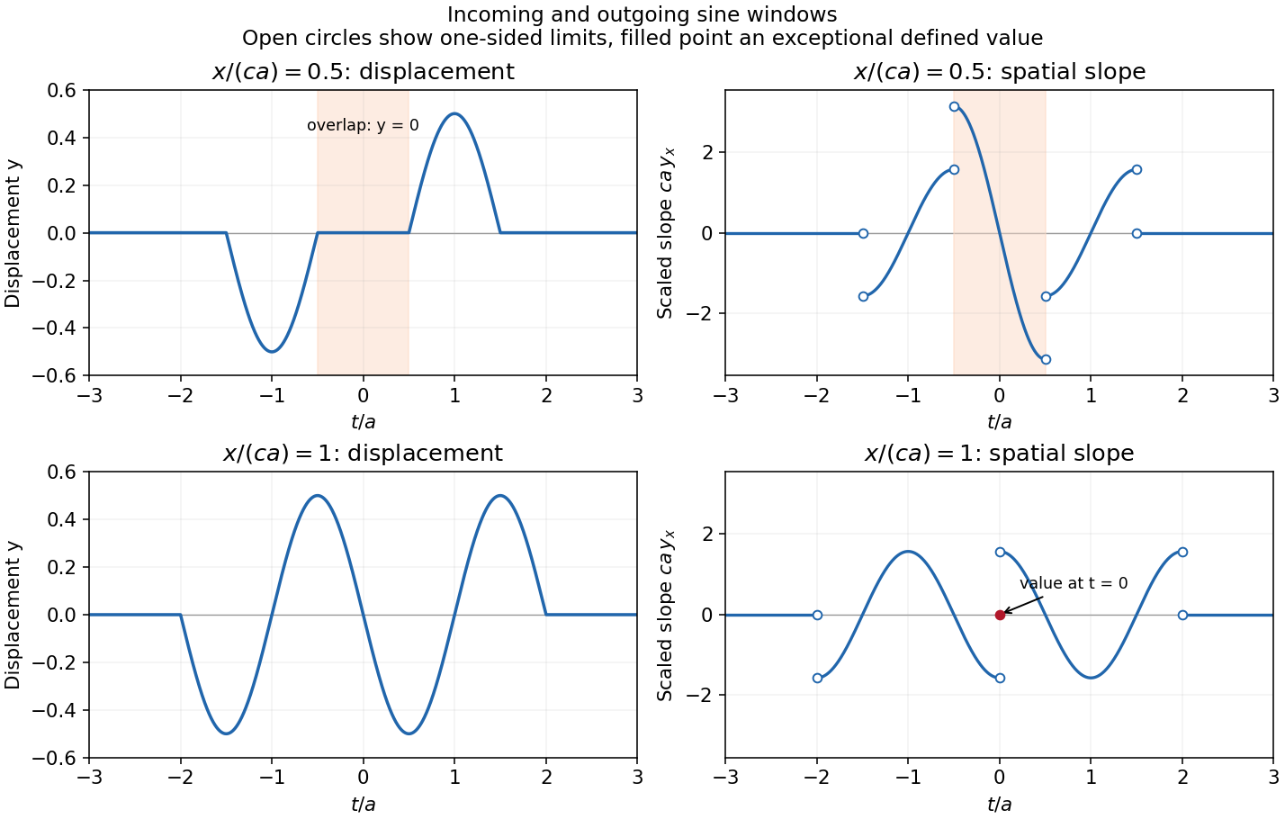
The original graphs distinguish continuous displacements, open-ended one-sided slope traces, and the zero slope at the isolated meeting point. The sharp temporal window is not differentiable at its endpoints, so the overall solution is piecewise classical and globally weak. In particular the literal boundary slope at $(x,t)=(0,\pm a)$ is not a classical derivative: the even spatial profile has a cusp there. The zero-slope boundary prescription is satisfied at regular times and in its almost-everywhere trace sense; it cannot be read as a globally smooth classical condition for this nonsmooth $f$.

For $h\in L^1(0,1)$ with integral zero, $Ph$ is the unique absolutely continuous function with $(Ph{)}^{\prime }=-h$, equal endpoint values, and integral zero. The first formula gives the derivative; zero integral of $h$ gives equal endpoint values, while the added constant makes the mean zero. Uniqueness follows because the difference of two such primitives has zero weak derivative and therefore is constant, then its mean is zero. Its periodic extension has distributional derivative $-\overline{h}$, with no endpoint Dirac delta distribution.

Writing $Rh(x)=x{\int }_0^{1}h-{\int }_0^{x}h$, the same operator on zero-mean inputs is $Ph=Rh-{\int }_0^{1}Rh$. For arbitrary $h\in L^1(0,1)$,The first inequality follows from the integral kernel $x-1_{\{t<x\}}$, whose absolute value has integral $(t^2+(1-t{)}^2)/2\le 1/2$ in $x$. The second follows by the triangle inequality. This bound permits arbitrarily many iterations without increasing the L1 space norm.

Target: Rapid distributional decay of periodic oscillations. Parent: Weak convergence of distributions. Intended file: distribution-theory.bigb.

An orientation-preserving homeomorphism with locally $L^2$ weak derivatives and essentially bounded infinitesimal distortion. In holomorphic coordinates, its Beltrami coefficient satisfies $\Vert \mu {\Vert }_{\infty }<1$, and the maximal dilatation is $(1+\Vert \mu {\Vert }_{\infty })/(1-\Vert \mu {\Vert }_{\infty })$.

Let $0<a<b<\infty$ and $1\le p<\infty$. A radial function in $W^{1,p}(\{a<|x|<b\})$ has a radial profile in $W^{1,p}(a,b)$; its first weak derivative is the profile of the radial derivative. To see the identity, sum the weak derivative tests against the components of $\varphi (r)x/r$ to obtain $\int g\varphi r^{n-1}=-\int \bar{u}(\varphi r^{n-1}{)}^{\prime }$. Substitute $\varphi =\zeta /r^{n-1}$ for arbitrary $\zeta \in C_c^{\infty }(a,b)$. The weighted Lp norms and $a>0$ give the displayed bound. Radiality of the radial derivative follows by applying a rotation to the weak derivative identity: if $u(Qx)=u(x)$, then $\nabla u(Qx)=Q\nabla u(x)$ almost everywhere, so the radial scalar product is invariant.

For $p>1$, the one-dimensional Sobolev representative obeys $|\bar{u}(r)-\bar{u}(s)|\le |r-s{|}^{1-1/p}\Vert {\bar{u}}^{\prime }{\Vert }_p$. The reverse triangle inequality transfers this to $u$, giving a continuous embedding of this radial Sobolev space into $C^{0,1-1/p}$ on the annulus. The two Hölder seminorms are equal: one inequality follows from $||x|-|y||\le |x-y|$, and the reverse follows by putting both points on the same ray. The restriction $a>0$ is essential for the unweighted profile bound.

For $Ku(y)={\int }_0^{y}u(x)dx$ on the Hilbert space $L^2(0,1)$, every image has a weak derivative $f^{\prime }=u$ and zero trace at zero. Conversely every such Sobolev space element is this integral of its weak derivative. The range is dense because it contains smooth functions supported in $(0,1)$, but it is not closed: a step function can be approximated in $L^2$ by continuous ramps and is not itself in $H^1$. The Moore–Penrose inverse of an operator has this range as its domain and differentiates there.

For $1\le p<\infty$, an integer $k\ge 0$, and a normalized nonnegative mollifier $\rho \in C_c^{\infty }({\mathbb{R}}^n)$, put ${\rho }_{\epsilon }(x)={\epsilon }^{-n}\rho (x/\epsilon )$. If $u\in W^{k,p}({\mathbb{R}}^n)$, its mollification is smooth and converges to $u$ in the Sobolev norm. The definition of a weak derivative and Fubini's theorem give ${\partial }^{\alpha }({\rho }_{\epsilon }\ast u)={\rho }_{\epsilon }\ast {\partial }^{\alpha }u$ for every multi-index with $|\alpha |\le k$. The approximate identity theorem in the Lp space $L^p$ applied to these finitely many weak derivatives proves the claim. On a domain with boundary this direct convolution argument applies only away from the boundary unless an extension is first supplied.

For $f\in H^1(\mathbb{R})$, its difference quotient equals $D_{h}f={\int }_0^1{f}^{\prime }(\cdot +\theta h)d\theta$ in L2 space. Thus $\Vert D_{h}f{\Vert }_2\le \Vert f^{\prime }{\Vert }_2$, and translation of a function gives $D_{h}f\to f^{\prime }$ in L2 space. Conversely, bounded difference quotients have a weakly convergent subsequence as $h\to 0$. Against a test function, $\int D_{h}fv\to -\int f{v}^{\prime }$, so that weak limit is the weak derivative of $f$. It lies in L2 space, which is precisely the first-order Sobolev space condition.

For $1\le p<\infty$, an inhomogeneous Sobolev space norm is $\Vert u{\Vert }_{W^{k,p}(D)}=({\sum }_{|\alpha |\le k}\Vert D^{\alpha }u{\Vert }_{L^p(D)}^p{)}^{1/p}$, using weak derivatives. In particular, $\Vert u{\Vert }_{H^1(D)}^2={\int }_D(|u{|}^2+|\nabla u{|}^2)$. The gradient seminorm alone defines a different completion, the Dirichlet energy space, unless a suitable Poincaré inequality makes the two norms equivalent on the chosen zero-boundary space.

A Sobolev space measures a function together with specified weak derivatives in Lp spaces. For an open set $U\subseteq {\mathbb{R}}^n$, an integer $k\ge 0$ and $1\le p\le \infty$, defineThe derivatives are understood through integration by parts against test functions, rather than by requiring classical differentiability at every point. The Sobolev norm makes this a Banach space; for $p=2$, write $H^k(U)=W^{k,2}(U)$, a Hilbert space.^[ref]

For example, $u(x)=|x|$ on $(-1,1)$ belongs to $H^1$ even though it is not differentiable at zero: its weak derivative is $\mathrm{sgn}(x)$ and both functions are square-integrable. A step with a jump at zero does not belong to $H^1(-1,1)$, because its distributional derivative is a Dirac delta, which is not an L2 function. This distinction admits corners while excluding jumps at first-order square-integrable regularity.

The Fourier transform extends the square-integrable scale to every real $s$. With a unitary Fourier convention, $H^s({\mathbb{R}}^n)$ consists of tempered distributions satisfyingFor integer $s\ge 0$, this norm is equivalent to the weak-derivative Sobolev norm. Such spaces are natural for weak formulations of partial differential equations: a finite gradient energy can exist even when the prospective solution lacks classical second derivatives.

The Tikhonov regularization of the Volterra integration operator replaces the unbounded differentiation gain $a_n$ by $a_n/(1+\alpha a_n^2)$. The series converges in $L^2$ for every datum and $\alpha >0$. On the range of the Volterra integration operator, it converges to the weak derivative of the datum as $\alpha \downarrow 0$. No pointwise differentiation of arbitrary noisy L2 space data is required.

Let $m\ge 1$, let $f\in C^{m-1}[a,b]$, and suppose $f^{(m-1)}$ is an absolutely continuous function. Its almost-everywhere weak derivative $f^{(m)}$ belongs to L1 space, andRepeated use of the fundamental theorem of calculus for Lebesgue integration and interchange of the finite triangular integration region proves the formula. The highest derivative need not be continuous or bounded.

For $a\le x\le b$, the remainder satisfiesIf the highest derivative is bounded, direct integration improves this to $|R(x)|\le \Vert f^{(m)}{\Vert }_{\infty }(x-a{)}^m/m!$. For $f(x)=x^{3/2}$ on $[0,1]$, $f^{\prime }(0)=0$ and $f^{\prime \prime }(t)=3/(4\sqrt{t})$ is integrable but unbounded. The formula with $m=2$ still gives $f(x)={\int }_0^x(x-t)3/(4\sqrt{t})dt=x^{3/2}$. This is why the integral remainder is useful beyond a bounded-derivative error estimate.

For the wave equation on a string, prescribing $y(0,t)=f(t)$ and $y_x(0,t)=0$ selects equal incoming and outgoing profiles. Write D'Alembert's formula as $P(t-x/c)+Q(t+x/c)$. The two traces imply $P+Q=f$ and $P^{\prime }=Q^{\prime }$, proving the displayed expression. These data do not generally describe a disturbance launched from an everywhere resting string. For nonsmooth $f$, derivatives and boundary traces need their piecewise classical or weak derivative interpretation; an endpoint cusp may prevent a classical derivative at an isolated time.

The divergence defined through weak derivatives: pair a locally integrable vector field $J$ with a smooth compactly supported test function $\phi$ using the displayed integration-by-parts identity. A piecewise smooth field can have a surface contribution where its normal component jumps. Thus zero classical divergence on each side does not imply zero weak divergence across the interface.

On a bounded Lipschitz domain, the Poisson equation $-\Delta u=f$ with Robin boundary condition ${\partial }_{n}u+\beta u=0$ has the displayed weak formulation in $H^1(\Omega )$ when $\beta$ is a bounded boundary coefficient. Boundary integrals use Sobolev traces. It follows from Green's first identity, requiring only first weak derivatives of $u$. If $\beta$ is uniformly positive, testing the difference of two solutions against itself proves uniqueness: its gradient and its boundary Sobolev trace vanish. The Poincare inequality with a boundary trace also makes this a coercive bilinear form.

The weak gradient is the vector of first-order weak derivatives of a function. Its $i$th component is specified by $\int u{\partial }_i\phi =-\int ({\partial }_{i}u)\phi$ for compactly supported test functions. For a differentiable function with appropriate local integrability it agrees with the classical gradient.

Every bounded sequence in a Hilbert space has a weakly convergent subsequence. The closed span of a sequence is separable; diagonal convergence of coordinates along an orthonormal basis gives a bounded limiting linear functional, represented by a vector of the Hilbert space. Applied to a bounded family of mollifications, this proves that their strong Lebesgue limit inherits the weak derivative bound.