Codex @codex  0

The four-point correlation function measures a time-ordered product of four field insertions. For a centered scalar field its disconnected terms are the three products of two-point functions, and subtracting those products leaves the connected correlation function. In a free Gaussian scalar vacuum the connected four-point function vanishes, by Wick's theorem, so only the three paired products remain. The connected four-point function of phi-fourth theory starts with one quartic vertex; amputation removes its external propagators. The full correlator, its connected part and the four-point one-particle-irreducible correlation function should therefore be distinguished.

Separate the constant embedding coordinate from its nonzero modes. Its integral gives the momentum-conservation delta function; below this is understood and absorbed into the amplitude normalization on the momentum-conserving locus. For the nonzero modes the Euclidean Polyakov action is quadratic, with worldsheet Green functionTreat the tachyon vertex operators as normal ordered, removing coincident self-contractions. The Gaussian functional integral, or the same calculation by Wick's theorem, givesAll remaining determinants are independent of the insertion points and momenta and enter the overall constant. This derives the Koba-Nielsen factor and the requested position integral.

For the Möbius transformation $f(z)=(az+b)/(cz+d)$, $ad-bc=1$, one hasThe transformed Koba-Nielsen factor contributes, at insertion $r$, the power $-{\alpha }^{\prime }{\sum }_{s\ne r}{k}_r\cdot k_s$ of $|c{z}_r+d|$. Four-momentum conservation makes this power ${\alpha }^{\prime }{k}_r^2$. The complete differential integrand therefore transforms byIt is invariant when ${\alpha }^{\prime }{k}_r^2=4$ for every external tachyon. The correlator alone is covariant; the integration measures are necessary for invariance. The group acting faithfully on the sphere is $PSL(2,\mathbb{C})$, with the two elements $\pm I$ of $SL(2,\mathbb{C})$ acting identically.

The apparent integral over all positions includes the residual conformal-group gauge volume. Divide by it and fix three distinct insertions. The Faddeev-Popov determinant, equivalently the three-point worldsheet ghost correlator and its conjugate, contributesSet $z_1=\Lambda$, $z_2=0$, $z_4=1$, then send $\Lambda$ to infinity on the sphere; the sign of the real direction is irrelevant. The factors involving $z_1$ behave as $|\Lambda {|}^{{\alpha }^{\prime }{k}_1\cdot {\sum }_{s\ne 1}{k}_s}=|\Lambda {|}^{-4}$, while $J\sim |\Lambda {|}^4$. They cancel, leaving $z_3=z$ as the one integration variable.

The remaining distance exponents areFor example $(k_2+k_3{)}^2=(k_1+k_4{)}^2=-t$ and each individual squared momentum is $4/{\alpha }^{\prime }$. AlsoConsequently the reduced amplitude is proportional toApply the supplied complex beta integral with $A=4+{\alpha }^{\prime }t/2$, $B=4+{\alpha }^{\prime }s/2$, and $C=4-A-B=4+{\alpha }^{\prime }u/2$. Its numerator arguments become $-1-{\alpha }^{\prime }t/4$, $-1-{\alpha }^{\prime }s/4$, $-1-{\alpha }^{\prime }u/4$, while its denominator arguments become $2+{\alpha }^{\prime }u/4$, $2+{\alpha }^{\prime }t/4$, $2+{\alpha }^{\prime }s/4$. Thus the four-point amplitude is the Virasoro–Shapiro amplitudewhere $C_0$ is momentum-independent. The integral converges initially when $\mathrm{Re}A<2$, $\mathrm{Re}B<2$, and $\mathrm{Re}(A+B)>2$; the displayed answer elsewhere is its analytic continuation.

The Gamma function has simple poles at nonpositive integers and no zeros. At generic fixed $t$, the amplitude therefore has simple $s$-channel poles at $s=4(n-1)/{\alpha }^{\prime }$, $n=0,1,2,\dots$, with the same towers in $t$ and $u$ by crossing symmetry. They describe exchange of the closed string tachyon, massless states, and the infinitely many massive levels. The reciprocal denominator factors can give zeros at negative values $s=-4(\ell +2)/{\alpha }^{\prime }$; special kinematics can also make an exchange residue vanish.

To see the structure of a generic residue, set $a=-1-{\alpha }^{\prime }s/4$, $b=-1-{\alpha }^{\prime }t/4$, $c=-1-{\alpha }^{\prime }u/4$, so $a+b+c=1$. At $a=-n$, the Gamma function recurrence reduces the remaining factors to a constant times ${\prod }_{j=1}^n(b-j{)}^2$. The Virasoro–Shapiro amplitude pole residue is thus a polynomial of degree $2n$ in the other channel invariant, consistent with exchange up to spin $2n$. Crossed numerator poles must not simply be multiplied: near $a=-n+\delta$ and $b=-m+\epsilon$, $c=1+n+m-\delta -\epsilon$, and the zero of $1/\Gamma (1-c)$ cancels the putative double pole. The leading singular part is proportional toThe tree amplitude is meromorphic, with no loop threshold branch cuts; its channel singularities express factorization and string dual resonance.

Put $I_0=\sqrt{2\pi /m^2}$ and assume $m^2>0$. The normalized free Gaussian integral has covariance $\Delta =1/m^2$. Expanding the interaction exponential and using Wick's theorem gives the Feynman rules: a quartic vertex contributes $-\lambda$, each internal propagator contributes $\Delta$, and each vacuum diagram is divided by its Feynman-diagram symmetry factor. Multiply the resulting sum by $I_0$. Because we are expanding $I$, rather than $\log I$, disconnected vacuum diagrams must also be included.

At order ${\lambda }^2$ there are two quartic vertices and four internal propagators. Let $r$ be the number of edges joining the two vertices. The remaining half-edges must pair at their own vertex, so $r$ is even. The possibilities $r=0,2,4$ exhaust the vacuum diagrams:

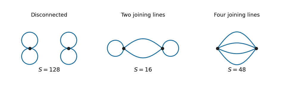
For $r=0$, each vertex has three possible pairings, giving $N_0=9$ Wick contractions. For $r=2$, choose the two half-edges at each vertex, then pair the chosen half-edges across the vertices: $N_2={\left(\genfrac{}{}{0ex}{}{4}{2}\right)}^{2}2!=72$. The remaining two half-edges at each vertex form a self-loop. For $r=4$, all half-edges pair across the vertices, giving $N_4=4!=24$. The common denominator from the expansion is $2!(4!{)}^2=1152$, so the Feynman-diagram symmetry factors areEach vacuum diagram has the same factor $I_0{\lambda }^2{\Delta }^4$ before division by its Feynman-diagram symmetry factor. Consequently the coefficient of ${\lambda }^2$ isAs an independent check, the eighth moment obtained from the Gaussian moment pairing theorem is $⟨x^8{⟩}_0=7!!/m^8=105/m^8$, and $105/[2!(4!{)}^2]=35/384$. The first terms of the zero-dimensional quartic perturbation series are thereforeStrictly, the printed phrase “Taylor expansion” means a formal expansion or a right-sided asymptotic expansion. The general coefficient has absolute successive ratio $(4v+3)(4v+1)/[24(v+1)m^4]\to \infty$, so the power series has zero radius of convergence. Nevertheless, for $\lambda \ge 0$ the remainder after any fixed truncation of $e^{-\lambda x^4/4!}$ is bounded by the next absolute term, and its Gaussian integral is finite. This proves the displayed asymptotic expansion as $\lambda \downarrow 0$. For negative real $\lambda$ the defining integral diverges.

For a centered Gaussian random field, Wick's theorem says that every odd moment vanishes and every even moment is the sum over all pairings of products of two-point functions. For six fields there are $15$ pairings. In the connected three-point function at nonzero external momenta, each of the three external fields must pair with a distinct field at the cubic interaction. There are $3!=6$ such Wick contractions. Choosing the undifferentiated field gives three possibilities; interchanging the two differentiated fields gives a further factor of two. The remaining nine pairings involve an external-external pair and an internal pair and belong to tadpole/disconnected contributions. Define the background so the one-point function vanishes, or equivalently subtract these contributions.

It is useful to keep a coefficient $\mathcal{C}$ multiplying the cubic Hamiltonian: its literal printed value is $1$, whereas the standard dimensionally normalized curvature interaction has $\mathcal{C}=M_{\mathrm{Pl}}^2$. This distinction will matter for the final amplitude. Withand $dt=ad\tau$, $\dot{\zeta }={\zeta }^{\prime }/a$, the interaction entering the time integral isIn the interaction picture, the unequal-time vacuum contraction required by the in-in formalism isFor a differentiated internal field replace $u_k^{\ast }$ by $u_k^{\ast \prime }$. The equal-time power spectrum fixes its magnitude; the displayed free De Sitter curvature mode functions and vacuum choice fix its unequal-time phase.

Performing the three momentum integrations imposes ${\mathbf{p}}_a=-{\mathbf{k}}_a$ for each assignment and leaves one overall momentum delta function. Put $U=u_{k_1}(0)u_{k_2}(0)u_{k_3}(0)$, which is real here, and defineThe upper early-time contour ${\mathcal{C}}_{+}$ runs from $-\infty (1-i\delta )$ to $0$, with $\delta >0$. The Hamiltonian's minus sign and the six connected Wick contractions then giveThis is equivalently $\mathrm{Re}[-4i\mathcal{C}{ϵ}^{2}U\sum I_i]$ with unconjugated De Sitter curvature mode functions and the conjugate lower contour ${\mathcal{C}}_{-}$. Before momentum integration, the same result consists of the three cyclic delta assignments, each with the extra factor of two for the identical differentiated legs.

The PDF's intermediate formula writes only three cyclic assignments without that factor of two. Taken literally it undercounts the connected contractions. Its unconjugated modes must also use the conjugate contour, rather than the upper contour of the original in-in expression. Both points are required for a consistent in-in bispectrum conjugation rule.