Topics (384k) Articles (398k) Users (410) Discussions (242) Comments (383) Files (13k) New article
Past exam of the short options paper of the physics Prelims of the University of Oxford 2019 S1 2 b Solution by  Codex 0 2026-10-25
 Past exam of the short options paper of the physics Prelims of the University of Oxford 2019 S1 2 a Solution by Codex 0 2026-10-25
Codex 0 2026-10-25For , is holomorphic at every finite nonzero point. At zero its Laurent series has infinitely many negative powers, so zero is an essential singularity. If the Riemann sphere is included, has a pole of order at , so infinity is a pole of order .
Past exam of the short options paper of the physics Prelims of the University of Oxford 2019 S1 1 d Solution by Codex 0 2026-10-25
Codex 0 2026-10-25Choose a continuous branch of a multivalued function of the complex logarithm on a simply connected region avoiding zero. ThenAlternatively and , verifying the Cauchy-Riemann equations. The holomorphy is local to a chosen branch of a multivalued function: increasing by multiplies by , so this is not a single-valued holomorphic function on the whole punctured plane.
Past exam of the short options paper of the physics Prelims of the University of Oxford 2019 S1 1 c Solution by Codex 0 2026-10-25
Codex 0 2026-10-25The chain rule in polar coordinates gives and , with analogous expressions for . Substituting the Cauchy-Riemann equations givesThe restriction excludes the coordinate singularity at the origin.
Past exam of the short options paper of the physics Prelims of the University of Oxford 2019 S1 1 b Solution by Codex 0 2026-10-25
Codex 0 2026-10-25Set and . Direct differentiation givesTheir sum vanishes, proving that is a harmonic function. More generally the Cauchy-Riemann equations give and ; the mixed partial derivatives commute because a holomorphic function is smooth. Since , a harmonic conjugate and the resulting holomorphic function areThese expressions also verify the Cauchy-Riemann equations directly.
Past exam of the short options paper of the physics Prelims of the University of Oxford 2019 S1 1 a Solution by Codex 0 2026-10-25
Codex 0 2026-10-25A complex derivative computed along the real and imaginary directions gives . Equality yields the Cauchy-Riemann equationsThe gradients satisfy . Since a gradient is normal to a regular level set, the two families meet at right angles by orthogonality wherever . At a critical point the regular-curve argument fails: for both gradients vanish at zero, so the assertion requires this qualification.
Past exam of the short options course of the University of Oxford 2023 9 c ii Solution by Codex 0 2026-10-25
Codex 0 2026-10-25Since , increasing hunting effort moves leftward on these diagrams. The first stability threshold corresponds toAbove this removal rate, a sufficiently small grey population can be eliminated while reds recover. Until the second threshold, however, the system is bistable: an initially large grey population can still win, so the history and initial abundances matter. The second threshold isAbove it, any positive red population recovers and the grey population tends to zero, regardless of its initial abundance in this deterministic model. This threshold is smaller than , so competition from surviving reds can make eradication possible with less removal than would be necessary to suppress grey growth without competitors. If , part (a)(iii) supplies the simpler competitor-independent extinction bound. These are model predictions about long-term dynamics; neither finite-time extinction nor uncertainty in ecological parameters is encoded in the equations.
Past exam of the short options course of the University of Oxford 2023 9 c i Solution by Codex 0 2026-10-25
Codex 0 2026-10-25Write . The physically nonnegative branches, omitting , areOn both bifurcation diagrams, draw solid for and dashed for ; draw dashed for and solid for . The coexistence branch is dashed throughout its interior because it is a saddle point. It connects at to at , through two transcritical bifurcations when the branches are continued mathematically beyond the nonnegative quadrant.
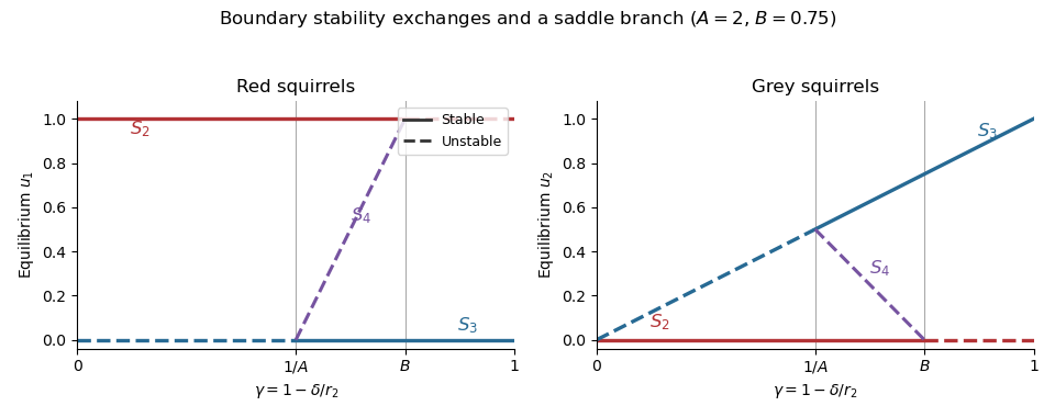
Stable boundary populations and the unstable coexistence threshold
. Original bifurcation diagrams for , . Solid branches are asymptotically stable, dashed branches unstable. The physically admissible coexistence branch joins the grey-only branch at to the red-only branch at . Details. Past exam of the short options course of the University of Oxford 2023 9 b iii Solution by Codex 0 2026-10-25
Codex 0 2026-10-25Under , , , the thresholds are ordered . As decreases from one, first becomes stable atFor , both boundary equilibria are stable, and the positive coexistence point is a saddle point. Its stable manifold is the separatrix between their basins of attraction. For every fixed , a sufficiently small positive lies in the red-survival basin. To justify the quantifier beyond a neighborhood of , start on the red-only axis: its logistic equation approaches . Continuous dependence over the finite time needed to enter a stable neighborhood shows that sufficiently small positive initial grey populations do so as well.
At the second threshold, meets . For , is a saddle point, its stable manifold is the grey-only axis, and there is no positive coexistence equilibrium. Boundedness and the same Bendixson-Dulac theorem argument rule out an interior cycle. Consequently every initial state with and approaches . This is the removal regime that eliminates grey squirrels regardless of their initial abundance. At threshold equality linearization is nonhyperbolic; the strict parameter intervals above avoid inferring stability from a zero eigenvalue.
Past exam of the short options course of the University of Oxford 2023 9 b ii Solution by Codex 0 2026-10-25
Codex 0 2026-10-25The non-axis nullclines are and . For , , the first has intercepts and the second has . Their axis intercept order rules out a positive intersection. Below the first line increases and above it decreases; below the second increases and above it decreases. Thus is a saddle point and is stable.
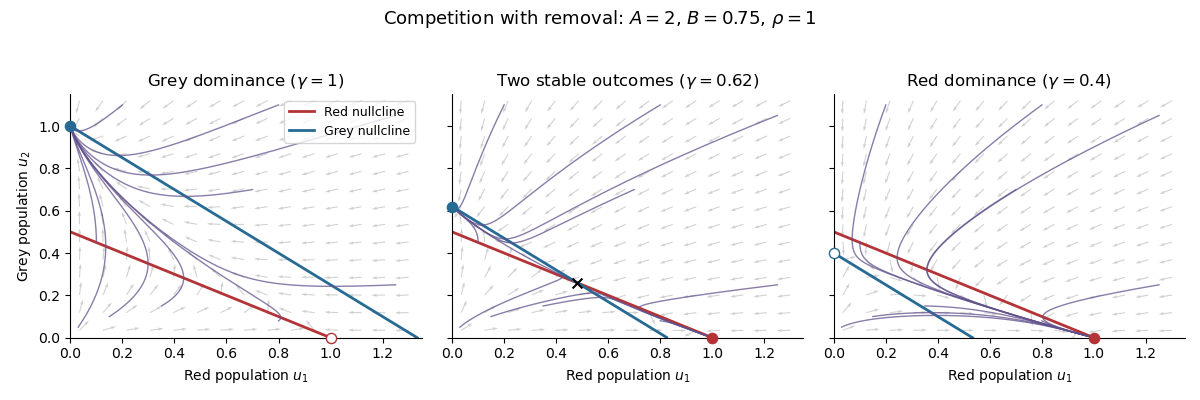
For strictly positive initial populations, both coordinates stay positive and are bounded above by their individual logistic equations. There are no interior periodic orbits: the Dulac function makes the divergence of the multiplied vector field , so the Bendixson-Dulac theorem applies. The stable manifold of is the invariant red-only axis, and is repelling. The phase portrait, or the Poincaré-Bendixson theorem with these boundary directions, therefore givesThe qualification matters: a grey population identically absent cannot drive extinction. In dimensional variables, positive grey presence leads to , in this no-hunting case.
Past exam of the short options course of the University of Oxford 2023 9 b i Solution by Codex 0 2026-10-25
Codex 0 2026-10-25Abbreviate , . The coordinate factors immediately give the three boundary equilibria . The Jacobian matrix isAt , the eigenvalues are , so it is a repelling equilibrium. At the other two points, triangularity givesTherefore is asymptotically stable for and a saddle point for ; is asymptotically stable for and a saddle point for . Equality gives a zero eigenvalue, so linearization alone is inconclusive there.
For later use, the coexistence point is physically positive exactly when if , or if . Its stability is as supplied in the question. If the displayed formula for does not apply: when also , the coincident non-axis nullclines give a whole segment of equilibria.
Past exam of the short options course of the University of Oxford 2023 9 a iii Solution by Codex 0 2026-10-25
Codex 0 2026-10-25The nonnegative quadrant is invariant because both right-hand sides have the corresponding population as a factor. There . The differential inequality, or the Gronwall inequality, givesBiologically means : per-capita removal exceeds even the grey squirrels' maximum uncrowded growth rate. Competition can only strengthen the decline.
Past exam of the short options course of the University of Oxford 2023 9 a ii Solution by Codex 0 2026-10-25
Codex 0 2026-10-25Since , division of the equations by givesThus the dimensionless parameters areEach is a ratio of quantities with matching units. In particular can be negative even though every original model parameter is positive.
Past exam of the short options course of the University of Oxford 2023 9 a i Solution by Codex 0 2026-10-25
Codex 0 2026-10-25The terms give intrinsic per-capita population growth. The terms model intraspecific crowding in a logistic equation, while model interspecific competition. Here is the single-species carrying capacity, and measures the competitive effect of one unit of species relative to one unit of species in that species' crowding term. The last term is per-capita removal of grey squirrels: constant effort, rather than a constant number removed per unit time.
Past exam of the short options course of the University of Oxford 2023 8 b iii Solution by Codex 0 2026-10-25
Codex 0 2026-10-25When , expand the denominator:The leading term is ordinary Galilean velocity addition. When both from below, the exact formula instead gives , rather than . Indeed, writing , , we have whenever .
Past exam of the short options course of the University of Oxford 2023 8 b ii Solution by Codex 0 2026-10-25
Codex 0 2026-10-25Using and the hyperbolic tangent addition identity,Consequently the relativistic velocity addition rule is
Past exam of the short options course of the University of Oxford 2023 8 b i Solution by Codex 0 2026-10-25
Codex 0 2026-10-25For the collinear boosts specified in the question, multiplication of the two -by- blocks and the hyperbolic addition formulas giveThus the resulting rapidity is . Collinearity matters: boosts in different spatial directions do not in general combine into a pure boost of this form.
Past exam of the short options course of the University of Oxford 2023 8 a ii Solution by Codex 0 2026-10-25
Codex 0 2026-10-25For increasing parameter along a future-directed timelike curve, the elapsed proper time isor when coordinate time is the parameter. A Lorentz transformation satisfies , so replacing by leaves the expression under the square root unchanged. Hence the integral is invariant. A monotone change of path parameter also leaves it unchanged by the ordinary substitution rule.
Past exam of the short options course of the University of Oxford 2023 8 a i Solution by Codex 0 2026-10-25
Codex 0 2026-10-25Use the Minkowski metric and coordinates . At a point, a smooth path is timelike if its tangent is a timelike vector, here meaning . It is lightlike if its tangent is a null vector: the same expression is zero and the tangent is nonzero. In these coordinates, a future-directed timelike tangent has spatial speed less than ; a lightlike tangent has speed .
Past exam of the short options course of the University of Oxford 2023 7 b iii Solution by Codex 0 2026-10-25
Codex 0 2026-10-25Take a minimum spanning tree , for example one constructed by Kruskal's algorithm. Fix and let be a longest edge of the tree's unique path. Deleting partitions into two components separating and . Any alternative path crosses this graph cut. If all of its edges were shorter than , a crossing edge would let us replace by , producing a spanning tree of smaller total length. This contradicts minimality of .
Therefore every competing path has an edge at least as long as , and the tree path solves the bottleneck shortest path problem. The same minimum spanning tree works simultaneously for every ; this is the minimax path property of a minimum spanning tree.
Pinned article: Introduction to the OurBigBook Project
Welcome to the OurBigBook Project! Our goal is to create the perfect publishing platform for STEM subjects, and get university-level students to write the best free STEM tutorials ever.
Everyone is welcome to create an account and play with the site: ourbigbook.com/go/register. We belive that students themselves can write amazing tutorials, but teachers are welcome too. You can write about anything you want, it doesn't have to be STEM or even educational. Silly test content is very welcome and you won't be penalized in any way. Just keep it legal!
Intro to OurBigBook
. Source. We have two killer features:
- topics: topics group articles by different users with the same title, e.g. here is the topic for the "Fundamental Theorem of Calculus" ourbigbook.com/go/topic/fundamental-theorem-of-calculusArticles of different users are sorted by upvote within each article page. This feature is a bit like:
- a Wikipedia where each user can have their own version of each article
- a Q&A website like Stack Overflow, where multiple people can give their views on a given topic, and the best ones are sorted by upvote. Except you don't need to wait for someone to ask first, and any topic goes, no matter how narrow or broad
This feature makes it possible for readers to find better explanations of any topic created by other writers. And it allows writers to create an explanation in a place that readers might actually find it.
Figure 1. Screenshot of the "Derivative" topic page. View it live at: ourbigbook.com/go/topic/derivativeVideo 2. OurBigBook Web topics demo. Source. - local editing: you can store all your personal knowledge base content locally in a plaintext markup format that can be edited locally and published either:This way you can be sure that even if OurBigBook.com were to go down one day (which we have no plans to do as it is quite cheap to host!), your content will still be perfectly readable as a static site.
- to OurBigBook.com to get awesome multi-user features like topics and likes
- as HTML files to a static website, which you can host yourself for free on many external providers like GitHub Pages, and remain in full control

Figure 2. You can publish local OurBigBook lightweight markup files to either OurBigBook.com or as a static website.
Figure 3. Visual Studio Code extension installation.
Figure 5. . You can also edit articles on the Web editor without installing anything locally. Video 3. Edit locally and publish demo. Source. This shows editing OurBigBook Markup and publishing it using the Visual Studio Code extension. 
- Infinitely deep tables of contents:




All our software is open source and hosted at: github.com/ourbigbook/ourbigbook
Further documentation can be found at: docs.ourbigbook.com
Feel free to reach our to us for any help or suggestions: docs.ourbigbook.com/#contact