The primes $2,5$ both work, with the zero residue as a solution. For every other prime, multiplicativity of the Legendre symbol and quadratic reciprocity giveThe first factor is positive for $p\equiv 1,7(\mathrm{mod}8)$; the second is positive for $p\equiv 1,4(\mathrm{mod}5)$. They must have the same sign. The Chinese remainder theorem therefore yields

For odd $p\ne 5$, quadratic reciprocity has no sign factor because $5\equiv 1(\mathrm{mod}4)$:The nonzero squares modulo $5$ are $1,4$, so the answer for odd primes is $p\equiv 1,4(\mathrm{mod}5)$. The excluded-prime wording also allows $p=2$, where $5\equiv 1$ has a square root. Thus the full answer is

For $p>3$, quadratic reciprocity givesThe second Legendre symbol is $1$ when $p\equiv 1(\mathrm{mod}3)$ and $-1$ when $p\equiv 2(\mathrm{mod}3)$. Combining it with the sign determined by $p(\mathrm{mod}4)$ shows that a quadratic residue occurs precisely for

If $p\mid n$, the field property forces $x=0$, giving exactly one solution. Otherwise, if $x_0$ is any solution, multiplication by $x_0$ is a bijection from the solutions of $z^k=1$ to those of $x^k=n$. Part (i) therefore givesThe two possibilities in the second line distinguish an empty fiber from a coset of the kernel of the power group homomorphism on ${\mathbb{F}}_p^{\times }$.

The multiplicative group ${\mathbb{F}}_p^{\times }$ is a cyclic group of order $p-1$, so choose a primitive root $g$. Every nonzero residue is uniquely $g^j$, with $j$ taken modulo $p-1$. The condition becomes $(p-1)\mid kj$. Writing $d=\gcd (k,p-1)$, its solutions are $j=0,(p-1)/d,\dots ,(d-1)(p-1)/d$. Zero is not a solution. Therefore the number isThis includes $p=2$. The cyclic group argument gives the exact count, whereas the bound of $k$ roots for a nonzero degree-$k$ polynomial over a field would only give an upper bound.

For $r>s$, $a>0$. When $0<a\le 1/4$, the roots of ${\mu }^2-\mu +a$ are real and lie strictly between zero and one. When $a>1/4$, they are a complex-conjugate pair of modulus $\sqrt{a}$. Thus the positive steady state is linearly asymptotically stable exactly when $0<a<1$, and unstable when $a>1$. Since $a=2s-2s^2/r$ increases strictly with $r$, the crossing occurs atAt the crossing,Every nonzero real linearized perturbation has period six. This establishes the intended linear stability threshold and linearized period six.

The nonlinear period-six claim in the printed paper does not follow, and is false as a local bifurcating-branch claim for this map. One can check this directly rather than infer a nonlinear period from the eigenvalues. At $r=r_c$ normalize $N_t=N^{\ast }(1+u)$, $N_{t-1}=N^{\ast }(1+v)$. The exact planar map isIts cubic Taylor expansion isHere is a concrete check of the sixfold return. Put $z=(u,v{)}^T$, $Q=u^2-uv+v^2$, andComposing the displayed cubic expansion six times cancels all quadratic terms and givesIn particularThe quartic coefficient is strictly negative. Hence, sufficiently near the equilibrium, every nonzero point has smaller $Q$ after six iterations: the critical nonlinear map has no nearby nontrivial period-six orbit, and the equilibrium itself is locally attracting despite its neutral linearization.

One can also rule out a branch of small period-six orbits on either side of the crossing. Normalize about the positive equilibrium at each nearby $r$, and put $\eta =a-1$. The derivative of the sixth power of $\left(\begin{array}{cc}1& -a\\ 1& 0\end{array}\right)$ at $a=1$ is $3I+K$. Smooth dependence on $r$ therefore givesThe leading matrix has determinant $(3\eta +\alpha Q{)}^2+3(\eta +\beta Q{)}^2$. Both terms could vanish with $Q>0$ only if $\alpha =3\beta$, butThus its norm on nonzero $z$ is bounded below by a positive constant times $(|\eta |+\Vert z{\Vert }^2)\Vert z\Vert$, and the smaller remainder cannot cancel it. There is no nearby nonzero solution of $F_{\eta }^6(z)=z$. The eigenvalues satisfy the nonresonance conditions through order four, their moduli cross outward with increasing $r$, and the cubic radial coefficient is negative. The standard Neimark–Sacker bifurcation theorem therefore gives a supercritical invariant closed curve. Its rotation is near the linear resonance $1/6$; it is not a local branch of exact period-six orbits.

Finally, the discrete population map does not preserve nonnegativity for arbitrary large lagged populations: $r/(1+b{N}_{t-1}^2)-\delta$ can be negative. The positive-equilibrium stability conclusions above are local and do not assume a global positivity property that the formula lacks.

Let $f(X,Y)=X[r/(1+b{Y}^2)-\delta ]$. At the positive steady state, $1+b(N^{\ast }{)}^2=r/s$, where $s=\delta +1$. The two partial derivatives areThe first-order Taylor expansion with $N_t=N^{\ast }+n_t$ therefore givesEquivalently, the linearization on $(n_t,n_{t-1})$ has matrix $\left(\begin{array}{cc}1& -a\\ 1& 0\end{array}\right)$ and characteristic polynomial ${\mu }^2-\mu +a$.

At a constant steady state $N_t=N$, the discrete equation reduces toWrite $s=\delta +1>1$. For $r<s$, no nonzero real root is possible, so zero is the only real steady state. For $r>s$ the real roots areThus there is exactly one strictly positive steady state, $N^{\ast }=\sqrt{(r-s)/(bs)}$. There are three real steady states in total, two of them nonnegative. At $r=s$ the only one is zero. This distinction keeps the positive-population statement separate from the count over all real numbers.

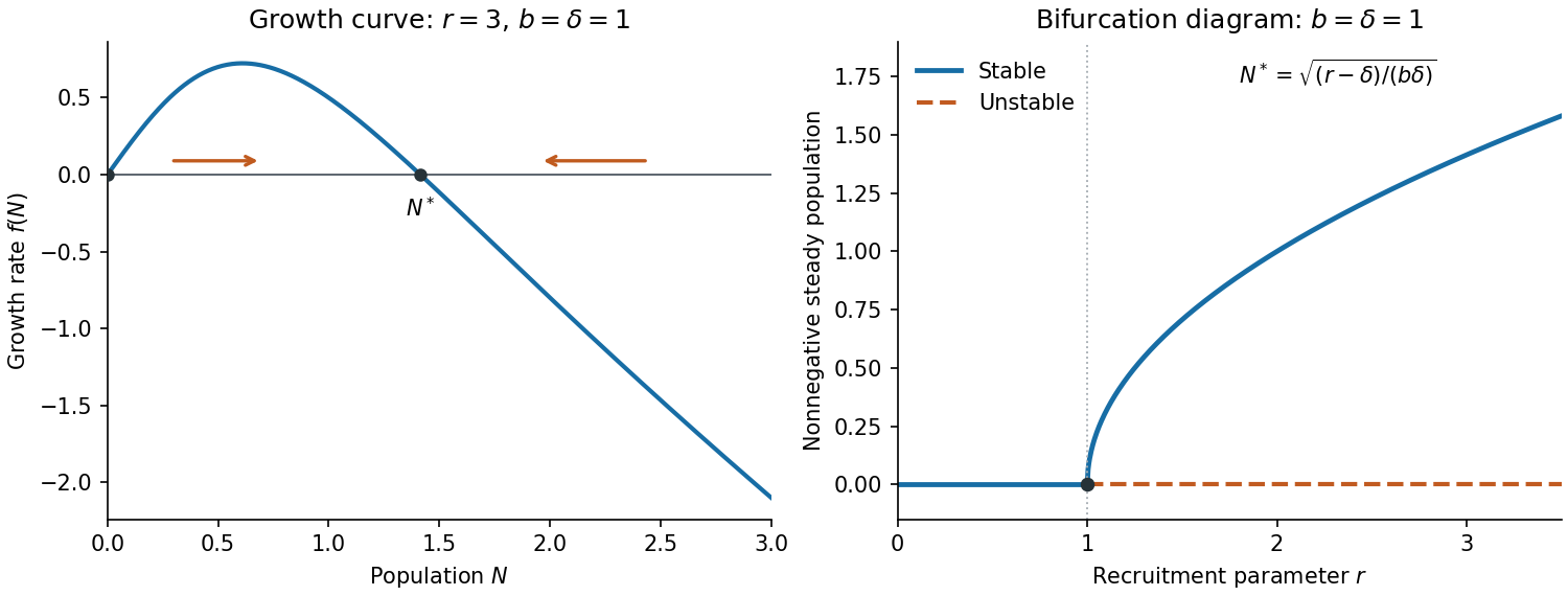
The nonnegative bifurcation diagram has the branch $N=0$ for every $r>0$, stable for $r<\delta$ and unstable for $r>\delta$. At $r=\delta$ the stable positive branch emerges:The figure in (iv) uses solid curves for stable steady states and a dashed curve for the unstable zero branch. At the meeting point the zero steady state is nonhyperbolic and attracts from the nonnegative side. If the equation is formally extended to negative $N$, there is also the symmetric branch $-N^{\ast }$, giving a supercritical pitchfork bifurcation; its negative half is omitted in the biological diagram. This qualification avoids calling the single nonnegative square-root branch a full pitchfork by itself.

For $r>\delta$, the sign of $f(N)$ is positive on $0<N<N^{\ast }$ and negative on $N>N^{\ast }$. Its graph passes through $0,N^{\ast }$, has positive initial slope $r-\delta$, and eventually behaves like $-\delta N$. The phase line therefore points toward $N^{\ast }$ from both sides.

The vector field is continuously differentiable, so solutions are unique. No positive solution crosses either equilibrium; one starting below $N^{\ast }$ increases and stays below it, and one starting above it decreases and stays above it. These bounded solutions exist for all forward time and have a limit. By continuity of $f$, any such limit must be a zero of $f$: otherwise the derivative would stay bounded away from zero near the limit. The increasing solution is bounded below by its strictly positive initial value, excluding zero; the decreasing one stays above $N^{\ast }$. ConsequentlyThe solution starting exactly at $N^{\ast }$ is constant. The zero initial condition remains at zero, which is why positivity is stipulated.

Linearizing at the positive steady state gives $n^{\prime }=f^{\prime }(N^{\ast })n$, so a small displacement decays as $n(t)=n(0)e^{-t/\tau }$. The recovery time of a stable equilibrium is thereforeAs $\delta \uparrow r$ with $r,b$ fixed, $N^{\ast }\to 0$ and $\tau \to \infty$. Thus the equilibrium population approaches extinction and recovers increasingly slowly after small perturbations. This is critical slowing down. Exactly at the threshold the leading equation is $N^{\prime }\sim -rb{N}^3$, which gives algebraic decay $N(t)\sim (2rbt{)}^{-1/2}$ instead of exponential recovery.

Write $f(N)=N[r/(1+b{N}^2)-\delta ]$. A steady state is a nonnegative zero of $f$. If $r<\delta$, the bracket is strictly negative for every $N\ge 0$, so only $N=0$ exists. If $r>\delta$, there are exactly two nonnegative steady states,For an autonomous scalar ordinary differential equation, a steady state with $f^{\prime }<0$ is locally asymptotically stable, while one with $f^{\prime }>0$ is unstable. HereAt the positive steady state, use $1+b(N^{\ast }{)}^2=r/\delta$ to obtainTherefore zero is stable for $r<\delta$ and unstable for $r>\delta$, whereas the positive steady state is stable whenever it exists. At the omitted equality $r=\delta$, $f(N)=-\delta b{N}^3/(1+b{N}^2)$; zero is nonhyperbolic but still attracts every nonnegative initial state.

The per-capita net growth rate is $r/(1+b{N}^2)-\delta$. Thus $r$ is the low-density per-capita birth or recruitment rate, $\delta$ is the constant per-capita death or removal rate, and $b$ controls density-dependent suppression of recruitment. Both $r$ and $\delta$ have units of inverse time; $b$ has units of inverse population squared. The population scale $b^{-1/2}$ halves the recruitment rate from its low-density value. Larger $b$ makes suppression important at smaller population sizes. These are interpretations of this phenomenological population dynamics model, rather than independently specified biological mechanisms.

For a photon, $m=0$ and $u=c$, so the result from (i) reduces toThis is relativistic aberration for a photon initially transverse to the boost. It also follows directly from $p_x^{\prime }=\gamma VE/c^2$ and $E^{\prime }=\gamma E$: the observed direction cosine is $c{p}_x^{\prime }/E^{\prime }=V/c$. The transverse observed speed is $c/\gamma =c\sin \varphi$, and the total photon speed is still $c$. If desired the observed photon energy is $E^{\prime }=E/\sin \varphi$ for $0<\varphi \le \pi /2$.

Let $V>0$ be the observer's speed, so its laboratory velocity is $-V{\mathbf{e}}_x$. The particle's laboratory speed along $+y$ follows from the energy–momentum relation:Here $E>m{c}^2$ because the massive particle is moving. Boosting to the observer's frame with velocity $-V$ gives, by the relativistic velocity-addition formula,Equivalently its four-momentum has $p_x^{\prime }=\gamma VE/c^2$, $p_y^{\prime }=p_y$. Thus $\tan \varphi =u/(\gamma V)$. Solving this equation, rather than using the Galilean transverse velocity, yieldsFor a strictly moving observer, $0<\varphi <\pi /2$. At $\varphi =\pi /2$ the limiting observer speed is zero; as $\varphi \downarrow 0$ it tends to $c$. The direction of the observer's velocity remains negative $x$; the displayed $V$ is its positive magnitude.

When both speeds are much smaller than $c$, expand the denominator of the velocity-addition formula:This is the Galilean transformation limit. For $0\le \beta =v/c<1$ and $0\le {\beta }^{\prime }=v^{\prime }/c<1$,If both $v,v^{\prime }\to c$ from below, the right side tends to zero, soNo sum of these subluminal speeds exceeds the speed of light.

By definition $v/c=\tanh \theta$ and $v^{\prime }/c=\tanh {\theta }^{\prime }$. Using the addition identity for the hyperbolic tangent and the rapidity sum from (i),Thus the velocity-addition formula isThe denominator is positive for the permitted subluminal signed velocities. For the nonnegative speeds in (iii), the composite is also nonnegative and remains below $c$.

In the common $ct,x_1$ plane, multiplication of the two Lorentz boost matrices givesThis follows from the addition identities for hyperbolic sine and hyperbolic cosine. The transverse coordinates are unchanged by both transformations. Consequently the rapidity of $\overline{O}$ relative to $O$ isThe signed rapidities add because both boosts use the same spatial axis and the stated matrix convention.

On the fixed parameter interval the integrand tends to $\cos \theta$ as $\kappa \to 0$ and is bounded by $\cos \theta$. The dominated convergence theorem, or uniform convergence here, givesThis equals Sam's time between departure and reunion. Physically, $dx/dt=-c\kappa \tan \theta$ tends uniformly to zero, so Alice's worldline approaches Sam's, and the time dilation disappears.

Differentiate the worldline with respect to $\theta$:Since $|\tan \theta |\le 1$ and $0<\kappa <1$, this is a future-directed timelike curve. The proper time element satisfies $c^{2}d{\tau }^2=c^{2}d{t}^2-d{x}^2$, henceAlice's total proper time is thereforeThis definite integral is an exact answer; it is an elliptic integral of the second kind. In notation $E(\alpha \mid m)={\int }_0^{\alpha }\sqrt{1-m{\sin }^{2}u}du$, it is $2\sqrt{2}TE(\pi /4\mid 1+{\kappa }^2)$. Although this parameter exceeds one, the integrand is real on the stated interval because its minimum squared value is $(1-{\kappa }^2)/2>0$.

The endpoint events have $(t,x)=(0,0)$ and $(2T,0)$. Sam stays at $x=0$ in his inertial frame, so his elapsed proper time is $2T$. For $\kappa >0$, the integrand is strictly less than $\cos \theta$ except at $\theta =0$, and ${\tau }_A<2T$.