A luminosity does not determine a stellar mass without a mass-luminosity calibration. Using the usual approximate main-sequence law $L/L_{\odot }=(M_s/M_{\odot }{)}^{\alpha }$ gives $M_s=3^{1/\alpha }{M}_{\odot }$. With $\alpha =3.5$, the numerical results areThe angular radius follows directly from $a(\mathrm{AU})/d(\mathrm{pc})$. Taking $\alpha =4$ changes these estimates by only a few percent, but the calibration must be stated. Hubble's 2.4 m aperture has visible-light diffraction scale $1.22\lambda /D\simeq 0.05$ arcsec at 500 nm, hundreds of times larger. The separation is therefore unresolved even before the severe star/planet contrast is considered.

Circular edge-on motion gives $V_s=2\pi a_s/P$ and center-of-mass balance gives $a_s=a{M}_p/(M_s+M_p)$. Eliminate $a$ using the preceding period relation:Thus $\boxed{M_p^3\simeq P{V}_s^3{M}_s^2/(2\pi G)}$ when $M_p\ll M_s$. For a non-edge-on orbit the measured velocity instead determines $M_p\sin i$ to this accuracy; neglecting eccentricity is also part of the stipulated model.

For two isolated point masses in a Newtonian bound orbit, $\boxed{P^2=4{\pi }^2{a}^3/[G(M_s+M_p)]}$, where $a$ is the relative orbit's semimajor axis. For a negligible planet mass, using years, astronomical units and solar masses gives $(P/\mathrm{yr}{)}^2=(a/\mathrm{AU}{)}^3/(M_s/M_{\odot })$. The mass in the denominator is the total gravitating mass, not the planet's mass alone.

In the cold underdense model, $1-v_g/c\simeq n/(2n_c)$ and ${\gamma }_{\varphi }^2\simeq n_c/n=500$. A relativistic electron slips through half an accelerating sinusoidal wavelength over $L_d\simeq {\gamma }_{\varphi }^2{\lambda }_p\simeq 8.35$ mm. For $E_z=E_0\sin \varphi$ and injection at the start of that half-cycle, integration over $0<\varphi <\pi$ givesInjection at the field crest and acceleration only to its next zero gives half this value, about 0.51 GeV; this explains a common factor-two convention in dephasing estimates. Multiplying the peak field by the entire dephasing length is instead an upper bound, not the sinusoid's actual integral. These are ideal wave-amplitude estimates: $a_0<1$ need not excite $E_0$, and finite pump depletion, pulse evolution and injection physics may reduce the gain. Without a specified nonlinear wake shape, the data warrant an order-GeV cold-wave upper scale, not a unique precision maximum for an actual experiment.

For linear polarization, $a_0=e{E}_L/(m_{e}c{\omega }_0)$ and $I={ϵ}_{0}c{E}_L^2/2$. Substitution gives $a_0\simeq 0.855{\lambda }_{\mu \mathrm{m}}\sqrt{I/(10^{18}\mathrm{W}\mathrm{c}{\mathrm{m}}^{-2})}\simeq 0.64$. Thus the specified peak electron quiver motion is at most mildly relativistic, not highly relativistic. Its quiver Lorentz factor is of order $\sqrt{1+a_0^2}\simeq 1.19$. The supplied 40 TW fixes a focal area through $P/I$, but does not increase $a_0$ once the intensity is specified. This exposes a limitation of assuming a strongly nonlinear, fully wavebreaking wake in the preceding estimates.

The laser driver should occupy at most roughly half a plasma period to excite the accelerating density response effectively. Interpreting pulse length as full significant spatial duration gives $\boxed{{\ell }_{\max }\sim {\lambda }_p/2\simeq 8.35\mu \mathrm{m},{\tau }_{\max }\sim 27.8\mathrm{fs}}$. If the source's $\sigma$ denotes the rms width of a Gaussian envelope instead, the resonant scale is commonly $k_p\sigma \sim 1$, or $\sigma \sim 2.66\mu$m and $8.9$ fs; full duration and rms width cannot be assigned the same numerical value without a pulse-shape convention. The robust condition is a sub-plasma-period pulse.

The supplied density is $4\times 10^{24}$ m${}^{-3}$. ThereforeThe cold relativistic field scale is $E_0=m_{e}c{\omega }_p/e\simeq 1.92\times 10^{11}$ V m${}^{-1}$, corresponding to an energy gradient $\boxed{e{E}_0\simeq 192\mathrm{GeV}{\mathrm{m}}^{-1}}$. It is an upper scale for the stipulated large-amplitude wave, not proof that the particular weak driver produces that field.

Use the explicit equation $n/n_c=0.002$; the surrounding phrase reverses the verbal ratio. It gives $n_c=2.0\times 10^{21}$ cm${}^{-3}$. From ${\omega }_0^2=n_c{e}^2/({ϵ}_0{m}_e)$,This is an underdense optical plasma. Treating the ratio as $n_c/n=0.002$ would instead contradict the specified underdense condition.

Equilibrium emittance obeys ${ϵ}_x=C_q{\gamma }^2{I}_5/(J_x{I}_2)$, with $I_5=\oint H(s)|\rho {|}^{-3}ds$, $H={\gamma }_x{\eta }^2+2{\alpha }_x\eta {\eta }^{\prime }+{\beta }_x{\eta }^{\prime 2}$. Thus reduce both bend angles and the dispersion invariant inside bends, rather than merely focusing to a small beam size elsewhere. The damping partition can also be adjusted within stability constraints.

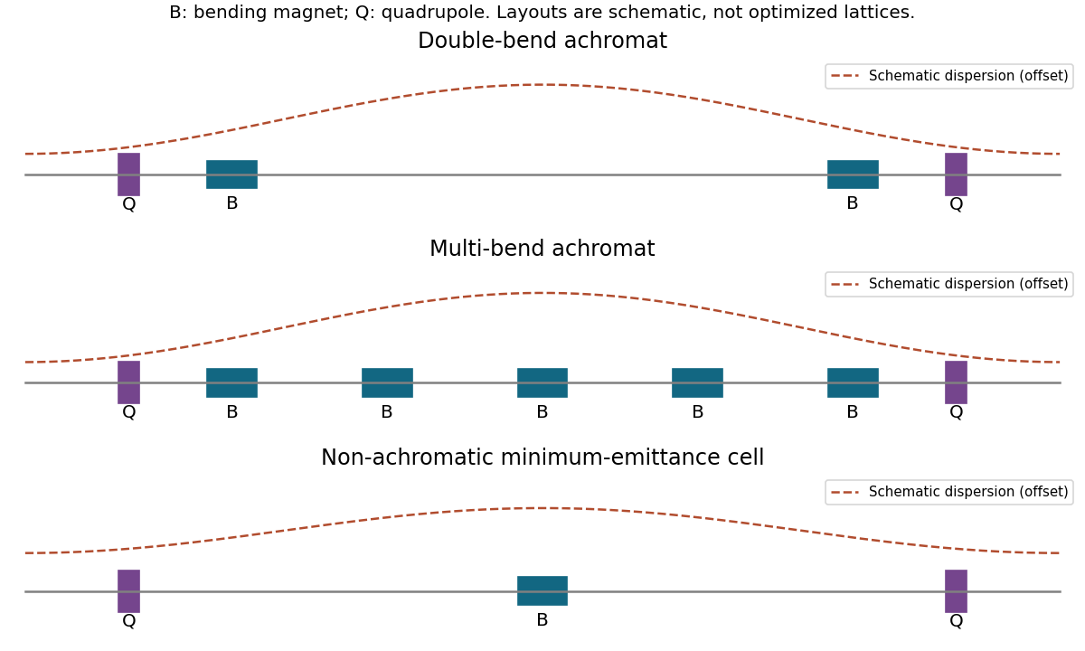
A DBA uses two bends and quadrupoles to return dispersion and its slope to zero at the cell boundaries; this provides dispersion-free insertion straights, at some emittance cost. A multi-bend achromat distributes the total angle over more weak bends and carefully controls the interior dispersion. A non-achromatic theoretical-minimum-emittance cell permits nonzero boundary dispersion and chooses the beta function and dispersion near a bend's optimum; longitudinal-gradient or reverse bends offer further control of radiation integrals. Strong focusing and dispersion suppression can increase natural chromaticity and sextupole demands, compromising dynamic aperture and momentum acceptance.

Doubling the number of identical-angle bends halves each angle. The minimum emittance scales as ${\theta }^3$, so it becomes $\boxed{0.240\mathrm{nm}\mathrm{rad}}$. At unchanged energy and unchanged individual magnet length, the bending radius doubles and field halves, giving $B=0.70$ T and $\boxed{E_c\simeq 4.19\mathrm{keV}}$.

At fixed stored current the loss per turn, proportional to $E^4\oint ds/{\rho }^2$, halves: twice as many equal-length bends each have one quarter of the original contribution. Total radiation power therefore halves. The spectrum softens by the factor-two critical-energy change. The characteristic high-energy vertical opening angle remains of order $1/\gamma$ at fixed energy, while each magnet's horizontal sweep halves. At a fixed absolute photon energy the normalized spectral position changes, so a claim that every angular distribution is identical would be too strong. Lower emittance also reduces the electron source size/divergence subject to the optical functions.

For identical uniform bends in an ideal double-bend achromat, the standard minimum is ${ϵ}_{x,\min }=C_q{\gamma }^2{\theta }^3/(4\sqrt{15}{J}_x)$, with bend angle $\theta =2\pi /48$ and $\gamma \simeq 3000/0.511$. Hence $\boxed{{ϵ}_{x,\min }\simeq 1.92\mathrm{nm}\mathrm{rad}}$. This uses the achromat constraint; the unconstrained theoretical-minimum-emittance coefficient is three times smaller.

The bending-magnet critical photon energy is $E_c=3\hslash c{\gamma }^3/(2\rho )\simeq 0.665E_{\mathrm{GeV}}^2{B}_{\mathrm{T}}$ keV, giving $\boxed{E_c\simeq 8.38\mathrm{keV}}$.

For fixed quadrupole fields and fractional momentum offset $\delta$, $q(\delta )=q_0/(1+\delta )$. Differentiate $\cos \mu =1-L_1{L}_2{q}^2/2$ at zero to obtain $d\mu /d\delta =-L_1{L}_2{q}_0^2/\sin \mu =-2\tan (\mu /2)$. ThusBoth transverse planes have the same natural result; the ring value is $N$ times this. It vanishes only in the zero-focusing limit, outside robust stable operation. Additional correcting elements, such as sextupoles where dispersion is nonzero, are required for zero corrected chromaticity.

For a periodic uncoupled lattice, $\mathrm{tr}M=2\cos \mu$ in the Twiss representation. Here $\cos \mu =1-L_1{L}_2{q}^2/2$, so bounded nondegenerate cell motion requiresThe zero-strength endpoint is only marginal and usually gives a drifting Jordan block. The phase advance increases from zero to $\pi$ on the positive-strength stable branch. Repeating the cell $N$ times gives ring eigenvalues $e^{\pm iN\mu }$ and tune $N\mu /(2\pi )$; it does not enlarge the stable strength interval. Integer ring phase advances can be resonance-sensitive in the presence of errors even when the ideal repeated matrix is bounded.

Take a reference point immediately before the focusing quadrupole and let matrices act on $(x,x^{\prime })$ from the right. With $q=1/f$, define $Q_F=\left(\begin{array}{cc}1& 0\\ -q& 1\end{array}\right)$, $Q_D=\left(\begin{array}{cc}1& 0\\ q& 1\end{array}\right)$ and $D(L)=\left(\begin{array}{cc}1& L\\ 0& 1\end{array}\right)$. One cell isIts determinant is one. A different starting point gives a conjugate matrix with the same trace and stability; the orthogonal transverse plane replaces $q$ by $-q$.

A plausible extension assuming gyromagnetic ratio two iswhere the spin projection is aligned with the charge-field sign. For spin one the lowest aligned mode has $E^2=m^2{c}^4-|e|\hslash |B|c$ at $p_z=0$. Above $|eB|>m^2{c}^3/\hslash$, this is negative: linear time evolution has exponentially growing/decaying modes, signaling an instability of the assumed background.

Spin alone does not fix a magnetic moment. The scalar and Dirac examples cannot establish this formula for every higher-spin particle; the stated instability belongs to the specified $g=2$ field model and its regime of applicability. Interactions and backreaction are needed to describe its eventual outcome.

Separate $x,z$ plane waves in the spinless equation. The transverse operator is $-{\hslash }^2{d}^2/d{y}^2+(p_x+eBy/c{)}^2$, the same shifted oscillator without a Pauli term. Its eigenvalues are $|e|\hslash |B|(2n+1)/c$. Thuswhich is the printed formula for $B>0$. The absence of the spin splitting is the substantive difference from the Dirac result.

Using $\epsilon =\hslash {\omega }_c(n+1/2)$ gives the charge-explicit resultFor $B>0$ the two spin signs are equivalently $m^2{c}^4+2m{c}^2[p_z^2/(2m)+\mu B(2n+1)\pm \mu B]$. Both positive and negative relativistic energy branches arise from this squared equation; an actual Dirac spinor must still be reconstructed from the coupled equations, especially at exceptional values where division by $E+m{c}^2$ is unavailable.

A simpler physical coordinate is $Y=y+p_{x}c/(eB)$. For ${\sigma }_3$ eigenvalue $s_z=\pm 1$, the equation becomes an oscillator of mass $m$, frequency ${\omega }_c=|eB|/(mc)$, and auxiliary energyIf the source's variable $\xi =(p_{x}c+eBy)/(\hslash c)=b_{B}Y$ is used literally, $b_B=eB/(\hslash c)$, then the same canonical oscillator form has $\boxed{M=m/b_B^2,\omega ={\omega }_c}$ and the same $\epsilon$. Because $\xi$ is an inverse length, this auxiliary $M$ is not a physical particle mass with ordinary mass dimensions; the rescaling must be carried through both kinetic and potential terms.

Eliminate the lower component to get $(E^2-m^2{c}^4)\phi =c^2(\sigma \cdot \Pi {)}^2\phi$. Since $[{\Pi }_x,{\Pi }_y]=ie\hslash B/c$, the Pauli identity gives $(\sigma \cdot \Pi {)}^2={\Pi }^2-e\hslash B{\sigma }_3/c$. Substitute the three momenta and rearrange:The spin-field sign follows from the charge convention and commutator, not an independent assignment.

In the source's Gaussian electromagnetic units, set $\mathbf{\Pi }=-i\hslash \nabla -e\mathbf{A}/c$ and take $\Phi =0$. ThenThe chosen gauge is independent of $x,z,t$, so simultaneous energy and canonical $p_x,p_z$ eigenstates justify the exponential ansatz. On the remaining spinors use ${\Pi }_x=p_x+eBy/c$, ${\Pi }_y=-i\hslash d/dy$, ${\Pi }_z=p_z$. The coupled equations are $(E-m{c}^2)\phi =c\sigma \cdot \Pi \chi$ and $(E+m{c}^2)\chi =c\sigma \cdot \Pi \phi$.