Use characteristic stellar values in the supplied radiative temperature gradient: $T_c/R\sim \kappa \rho L/(R^2{T}_c^3)$. Hence $L\propto T_c^{4}R/(\kappa \rho )$. With Kramers opacity, $\kappa ={\kappa }_0\rho T_c^{-3.5}$,Hydrostatic support by an ideal gas gives $T_c\propto \mu M_s/R$, or $R\propto \mu M_s/T_c$. Substitution then yieldsThe result assumes homologous density and temperature profiles, comparable structural constants, gas-pressure support and radiative transport throughout. It is not simultaneously an electron-scattering-opacity result; replacing Kramers opacity changes the exponents. Convection, degenerate cores or a different opacity regime limit quantitative application to real evolved helium stars.

Opacity is the extinction cross section per unit mass for radiation; a frequency-dependent value ${\kappa }_{\nu }$ gives $d{I}_{\nu }/ds=-{\kappa }_{\nu }\rho I_{\nu }$ when emission is considered separately. Stellar radiative diffusion generally uses an appropriately weighted Rosseland mean opacity. The associated local mean free path is of order $1/(\kappa \rho )$.

At sufficiently high temperature the material is highly ionized, and scattering by free electrons is often dominant for ordinary stellar densities and photon energies well below the electron rest energy. Bound-bound and bound-free absorption weaken as bound electrons disappear; free-free absorption can still matter depending on temperature and density. Thus “high temperature” does not fix the dominant opacity at every possible density. The next part explicitly imposes a Kramers absorption law as a separate scaling model.

The radiation pressure at a photospheric temperature near $5800$ K is only about $0.3$ Pa. For an illustrative photospheric gas density $3\times 10^{-4}\mathrm{kg}{\mathrm{m}}^{-3}$ and mean molecular weight near $1.3$, the ideal gas pressure is about $10^4$ Pa. Thus gas pressure dominates those outer layers by many orders of magnitude. Both the temperature and density are needed: low temperature alone is not a complete comparison.

For homologous stars, hydrostatic and ideal-gas estimates give $T\sim \mu m_{H}GM/(k_{B}R)$ and $\rho \sim M/R^3$. Thereforewith a structural coefficient independent of mass only under the homology assumption. As mass rises, radiation becomes increasingly important. A rough solar interior normalization of $10^{-3}$-$10^{-2}$ suggests equality after a mass increase by tens, while realistic radiation-dominated structure and composition shift the scale; stars of order $10^2{M}_{\odot }$ are a useful estimate for strong radiation support. The very small photospheric ratio must not be used as a universal normalization for their whole interiors.

Radiation also transfers outward momentum. Comparing radiative acceleration $\kappa L/(4\pi r^{2}c)$ with gravity gives the Eddington luminosityNear this scale, radiatively driven winds and envelope instabilities can remove matter or impede further accretion. Opacity, composition, rotation, mass loss and formation history affect the limiting stellar mass. The Eddington condition is a luminosity-to-mass constraint, not a unique composition-independent maximum stellar mass.

Multiply hydrostatic equilibrium by $4\pi r^{3}dr$ and integrate from centre to surface. Integration by parts, neglecting external surface pressure, givesFor an ideal gas with a constant adiabatic index, $U=\int PdV/(\gamma -1)$. ConsequentlyA fully ionized, nonrelativistic monatomic gas has $\gamma =5/3$, provided gas rather than radiation or degeneracy dominates the thermal equation of state. It then obeys $\boxed{2U+\Omega =0}$ and $E=U+\Omega =-U=\Omega /2$.

Added nuclear heat initially raises pressure and causes expansion. The expansion makes gravitational energy less negative and can lower the temperature of the self-gravitating gas, reducing the temperature-sensitive fusion rate. Conversely, a small contraction can raise the core temperature and increase burning. This negative feedback explains stable main-sequence burning in an ordinary nondegenerate stellar core; a degenerate core need not respond the same way.

Before hydrogen ignition, a cloud loses energy by radiation and contracts. Its gravitational energy decreases; for the ideal-gas virial relation, roughly half the released binding energy heats the gas and half is radiated. Heating continues until nuclear reactions can balance the luminosity, explaining the Kelvin-Helmholtz phase of pre-main-sequence evolution.

The effective adiabatic response varies with ionization, molecular dissociation, radiation pressure and degeneracy. Partial ionization can absorb compression energy and lower the local first adiabatic exponent below $4/3$, encouraging compressibility, convection and pulsational instability. A local outer layer with $\gamma \le 4/3$ does not by itself prove global collapse: ordinary stars have ionization layers of that kind. The dynamical stability criterion concerns a suitable pressure-weighted global response and its coupling to the eigenmode; an extended star with an effectively global exponent below $4/3$ can be dynamically unstable.

A thin spherical shell of thickness $dr$ has mass $4\pi r^2\rho dr$. Balancing its inward gravitational force with the pressure difference across its faces givesFor a transparent estimate take constant density $\rho =3M_{\odot }/(4\pi R_{\odot }^3)$ and negligible surface pressure. Then $M_r=M_{\odot }{r}^3/R_{\odot }^3$, so integration givesCombining with the ideal gas law and $\mu \simeq 0.6$ yields $T_c\simeq \mu m_{H}G{M}_{\odot }/(2k_B{R}_{\odot })\simeq 7\times 10^6$ K. The less specific virial scaling gives $T_c\sim \mu m_{H}G{M}_{\odot }/(k_B{R}_{\odot })\sim 10^7$ K.

The real Sun is strongly centrally concentrated: a uniform-density model substantially underestimates central pressure and is not a detailed solar model. Its value is a justified scale estimate, while more realistic structure produces central temperatures of order $1.5\times 10^7$ K and central pressures of order $10^{16}$ Pa. Hydrostatic equilibrium alone does not uniquely determine both profiles without an equation of state and a density/thermal model.

Adiabatic photon redshifting gives $T\propto a^{-1}$. Using the stipulated temperatures,In the flat dust approximation of part c, $t=t_0{a}^{3/2}$, so $t_{\mathrm{rec}}\simeq (2/3H_0)1000^{-3/2}\simeq 2.75\times 10^5$ years. This approximation omits the significant radiation contribution near the actual recombination epoch.

The elementary travel-distance estimate is $c{t}_{\mathrm{rec}}\simeq 8.4\times 10^4$ pc, whose corresponding comoving scale today is about $84$ Mpc. In an expanding universe, however, that is not the exact proper particle-horizon radius. Integrating the null geodesic givesfor dust. Thus the proper horizon at this epoch is about $0.25$ Mpc and its present comoving size about $250$ Mpc. The factor three accounts for expansion during light propagation. These scales describe the limited causal domain in the simple decelerating model. The near-uniform CMB temperature across much more widely separated last-scattering regions motivates the horizon problem; the question's rough $ct$ estimate and the exact dust horizon should not be conflated.

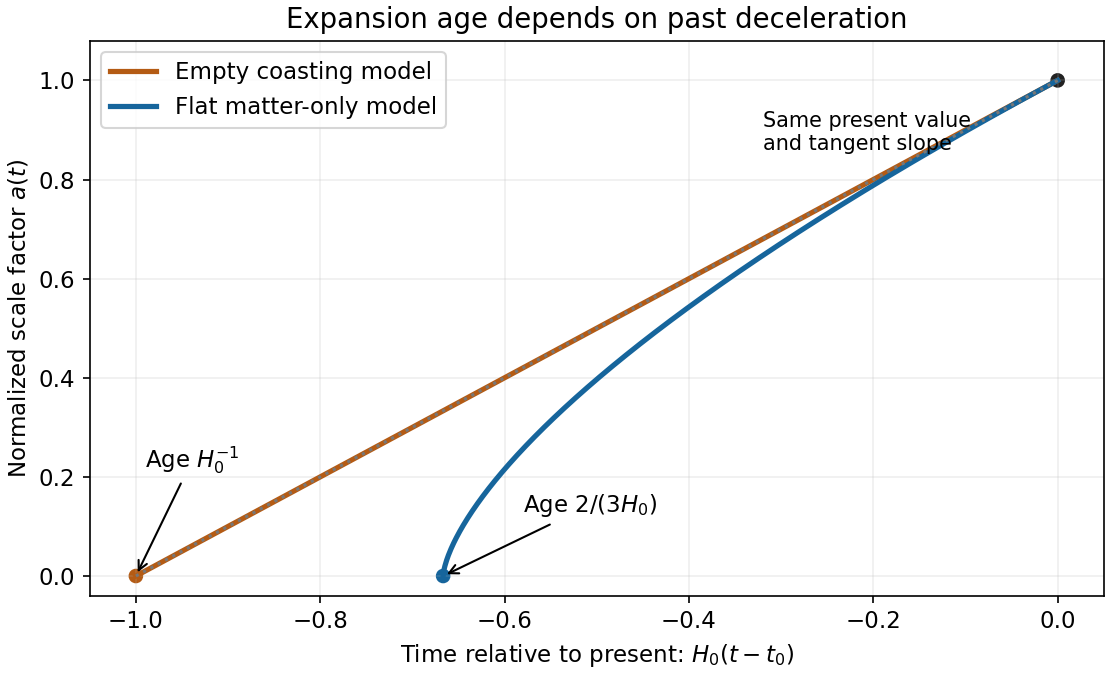
With zero curvature and no cosmological constant, the present normalization requires ${\Omega }_M=1$. Thus $\dot{a}=H_0{a}^{-1/2}$, and choosing the big bang as $t=0$ givesFor an empty expanding model, ${\Omega }_k=1$ and the curvature must be negative. The equation becomes $\dot{a}=H_0$, givingThe latter is the Milne slicing of flat spacetime; its zero-scale-factor origin is not a matter-density curvature singularity. In the matter model, gravity decelerates expansion, so the earlier slope was greater than the present slope and the same present size was reached in less time. With the stipulated $H_0$, the two model ages are approximately $8.69$ and $13.0$ Gyr.

For conserved nonrelativistic matter, ${\rho }_M={\rho }_{M0}{a}^{-3}$, where $a=R/R_0$ and $a_0=1$. Substitution into the Friedmann equation giveswithThe source writes the dimensionless normalized factor as $R$ in its final expression; this is equivalent to setting $R_0=1$ consistently in the curvature coefficient. Evaluating today gives ${\Omega }_M+{\Omega }_k+{\Omega }_{\Lambda }=1$. Here the printed $\Lambda$ already has dimensions of inverse time squared. If the cosmological constant is instead defined geometrically with inverse-length-squared units, replace this $\Lambda$ by ${\Lambda }_{\mathrm{geom}}{c}^2$.

The curvature constant specifies the intrinsic spatial curvature of homogeneous constant-time slices. Positive curvature has spherical geometry, zero curvature Euclidean geometry, and negative curvature hyperbolic geometry. A conventional coordinate normalization uses $k=+1,0,-1$, with the scale factor carrying the curvature radius; rescaling that factor changes the numerical magnitude assigned to a dimensional curvature coefficient.

The sign alone does not determine the future expansion once a cosmological constant is admitted. Nor does negative or zero local curvature by itself determine the global topology: quotient spaces can share the same local curvature.

Let $I$ denote a characteristic surface brightness and ${\rm Y}=M/L$ the relevant dynamical mass-to-light ratio. With comparable profiles, $L\propto I{R}^2$ and $M\propto V^{2}R/G$. Eliminating $R$ givesIf both $I$ and ${\rm Y}$ are independent of speed, converting luminosity to magnitude gives $M_V=\text{constant}-10{\log }_{10}V$. The empirical coefficient $-8$ instead means $L\propto V^{3.2}$, and thereforeFor constant surface brightness this requires ${\rm Y}\propto V^{0.4}$; for constant mass-to-light ratio it requires $I\propto V^{0.8}$. A mixture of these changes, including varying stellar populations or dark-matter fractions, can give the same observed slope. The simple derivation assumes comparable characteristic radii and structural coefficients.

Using the same luminosity estimate, the distance modulus is $12.5-(-22.49)=34.99$, implying $D\simeq 99.4$ Mpc. Pure Hubble expansion at that distance predicts about $7450\mathrm{km}{\mathrm{s}}^{-1}$. The measured velocity therefore impliesIts line-of-sight peculiar velocity is toward us, of the order expected for orbital motions in a rich galaxy cluster. A galaxy falling toward a cluster centre from its far side could have this sign. Its actual front/back location or three-dimensional orbit is not determined without the cluster's mean velocity, distance and projected position. Tully-Fisher scatter and the assumption of identical luminosities also limit that inference.

The effective radius is one tenth of the optical outer radius: $R_e\simeq 2.13$ kpc. A flat rotation speed then gives $M_{\mathrm{dyn}}(<R_e)\simeq 4.9\times 10^{10}{M}_{\odot }$. Half the luminosity, with the same mass-to-light ratio, implies $M_{\mathrm{luminous}}(<R_e)\simeq 4.9\times 10^{10}{M}_{\odot }$.The concentration of light into a small fraction of the optical radius suggests a high-surface-brightness, centrally concentrated disk galaxy, plausibly an early-type spiral or lenticular with a substantial bulge. The kinematic and photometric data do not uniquely distinguish those morphologies. Disk geometry, an unknown inclination correction, or a varying stellar mass-to-light ratio would alter the exact numerical inner comparison.

At this small redshift, $D\simeq cz/H_0\simeq 20.0$ Mpc. The outer angular radius gives $R_{\mathrm{out}}\simeq D\theta \simeq 21.3$ kpc. Approximating the dynamical mass by a spherical equivalent,The supplied Tully-Fisher relation gives $M_V\simeq -22.49$, and hence $L_V\simeq 9.9\times 10^{10}{L}_{V,\odot }$. Treating the population as solar-like gives the estimate ${{\rm Y}}_V\simeq 1M_{\odot }/L_{V,\odot }$, soThe dynamical estimate exceeds that by about a factor of five; a massive extended dark-matter component is the natural interpretation. Solar-like spectra do not exactly fix the population mass-to-light ratio, and a disk is not spherical, but order-unity corrections do not remove this large outer mass excess under the stated estimate.

The numbered features in the original colour-magnitude diagram have the following interpretation.

Continuous star formation explains the coexistence of newly formed massive main-sequence stars with evolved low-mass remnants; interpreting a single sharp turnoff as the age of a coeval cluster would be inappropriate here.

If radiation dominates the central pressure, equate $P_c\sim G{M}_{\ast }^2/R_{\ast }^4$ to $a{T}_c^4/3$. This givesAt roughly fixed burning temperature, the corresponding mass-radius scaling is $R_{\ast }\propto M_{\ast }^{1/2}$, rather than the gas-pressure estimate $R_{\ast }\propto M_{\ast }$. Radiation pressure alone does not determine a unique radius at a specified mass: a thermal or nuclear-burning condition is still needed to specify $T_c$. The relation is a homology estimate, not a universal exact law for all massive stars.

Integrating $dP/dr=-G{M}_r\rho /r^2$ in order of magnitude, with $\rho \sim M_{\ast }/R_{\ast }^3$, givesThe ideal gas law independently gives $P_c\sim M_{\ast }{k}_B{T}_c/(\mu m_H{R}_{\ast }^3)$. Equating the two estimates yieldsFor similar composition and an approximately fixed hydrogen-burning central temperature, $R_{\ast }\propto M_{\ast }$. Calibrating this rough relation on the Sun and using part a gives a nominal mass range of about $0.05$ to $5M_{\odot }$.

The endpoint luminosity ratio is $10^8$, whereas the inferred mass ratio is about $10^2$, giving $L\propto M^4$ across that range. The exponent is therefore consistent at this schematic level. The solar normalization and individual endpoint masses are much less reliable: using the luminosity relation itself gives approximately $0.1$ to $10M_{\odot }$. Central temperatures are not truly constant, low-mass stellar structure differs, and the uncorrected $V$ luminosities in the diagram are not bolometric. These limitations prevent treating the rough radius-based masses as a contradictory precision measurement.

The distance modulus at $100\mathrm{pc}$ is five magnitudes. Thus the two approximate main-sequence endpoints read from the original figure, $m_V\simeq 0,20$, correspond to $M_V\simeq -5,15$. With the given solar reference,Use the figure's approximate endpoint effective temperatures $25,000$ K and $2500$ K. If $V$-band luminosity is used as a rough bolometric proxy, the Stefan–Boltzmann law givesTaking $T_{\odot }\simeq 5800$ K givesThese are schematic estimates, not precision radii. The diagram supplies $V$ magnitudes rather than bolometric luminosities, and hot and cool endpoints need different bolometric corrections. The exact range cannot be recovered without those corrections; the quoted values state the intended approximation explicitly.

If the driver can be fully depleted with transformer ratio six, the largest ideal witness gain from a $62.5$ GeV proton is $375$ GeV. Each lepton then hasFor equal opposing electron and Positron beam energies,The associated ideal population ratio would be $N_p/N_e=6$. This energy-budget ceiling ignores wake-generation and transfer losses, staging limits, emittance preservation and the difficulty of accelerating both charge signs with suitable focusing. It is the consequence of the stipulated transformer-ratio bound, not a prediction of an achievable upgrade.

The mean witness gradient must be $112.5\mathrm{GeV}/1.1\mathrm{m}\simeq 102\mathrm{GV}{\mathrm{m}}^{-1}$. To turn this into a density estimate, assume an accelerating wake amplitude of order the cold plasma wave-breaking scale,Eliminating ${\omega }_p$ givesThe associated plasma wavelength is about $31$ micrometres, illustrating why a short driver structure is required. The given length and energy gain do not uniquely fix density without an assumption about wake amplitude relative to the plasma scale. Driver shape, beam loading, relativistic wave-breaking corrections and matching to a Positron witness are substantive additional issues; the estimate is a scale calculation, not a completed accelerator design.

For ideal transfer of the proton bunch's kinetic energy to the witness bunch,ThusThis is a minimum driver population for unit efficiency and full depletion under the stated energy budget. If only a fraction $\eta$ is usefully transferred, the required ratio becomes $1.8/\eta$. The equality to the transformer ratio uses the same ideal matching assumption as part b.