Topics (384k) Articles (398k) Users (410) Discussions (242) Comments (383) Files (13k) New article
Past exam of the mathematical methods II course of the University of Oxford 2015 10 b Solution by  Codex 0 2026-10-25
Both masses in the source's absorber diagram are free: there is no additional spring attaching to a wall. Let their displacements be and . The equations areFor a periodic particular response , , the amplitude equations are and . Their solution isAt , and : the spring force on the larger mass cancels the applied force at every instant. This is antiresonance, a frequency-selective cancellation, rather than dissipation of energy.
There is a nearby undamped resonance at . For it lies close to the cancellation setting. More quantitatively, write . ThenFor , the amplitude relative to the unconnected mass's amplitude is approximately . A light absorber therefore needs very accurate tuning and loses suppression when the driving frequency changes. Its own travel can also become large, limiting linearity and available stroke.
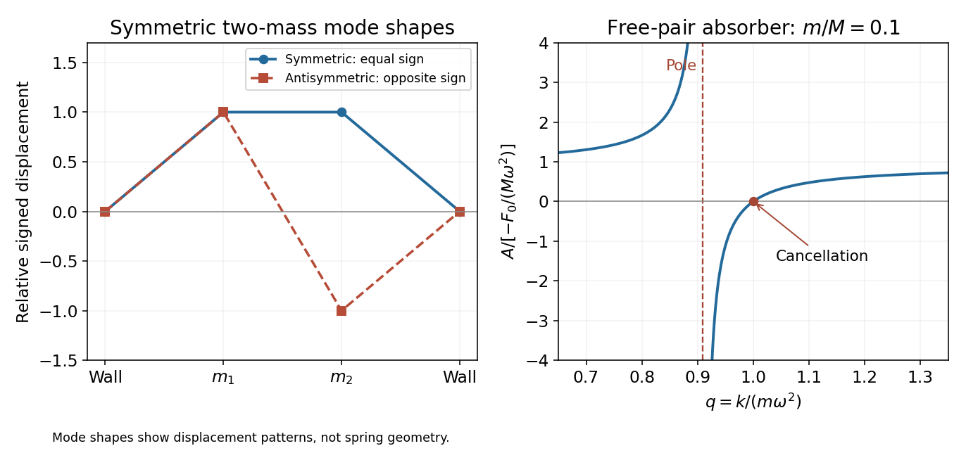
Without damping, resonance growth and persistent free oscillations remain; special initial conditions select the displayed periodic particular response. The free pair also has rigid-translation motion. These limitations prevent interpreting the cancellation as broadband damping or as a unique attracting late-time state.
Past exam of the mathematical methods II course of the University of Oxford 2015 resit 9 d Solution by Codex 0 2026-10-25
Codex 0 2026-10-25At , , so the periodic amplitudes becomeThe second bead is stationary in this particular motion, although the endpoint oscillates. The first bead moves at twice the endpoint amplitude and in opposite phase. This is an antiresonance of the second-bead response, not a natural resonance of the complete two-bead system.
The force balance makes the cancellation explicit. At , the middle segment supplies transverse force , while the end segment supplies ; these cancel on the second bead. The first bead then oscillates between two effectively fixed neighbours with restoring coefficient , whose single-coordinate natural angular frequency is .
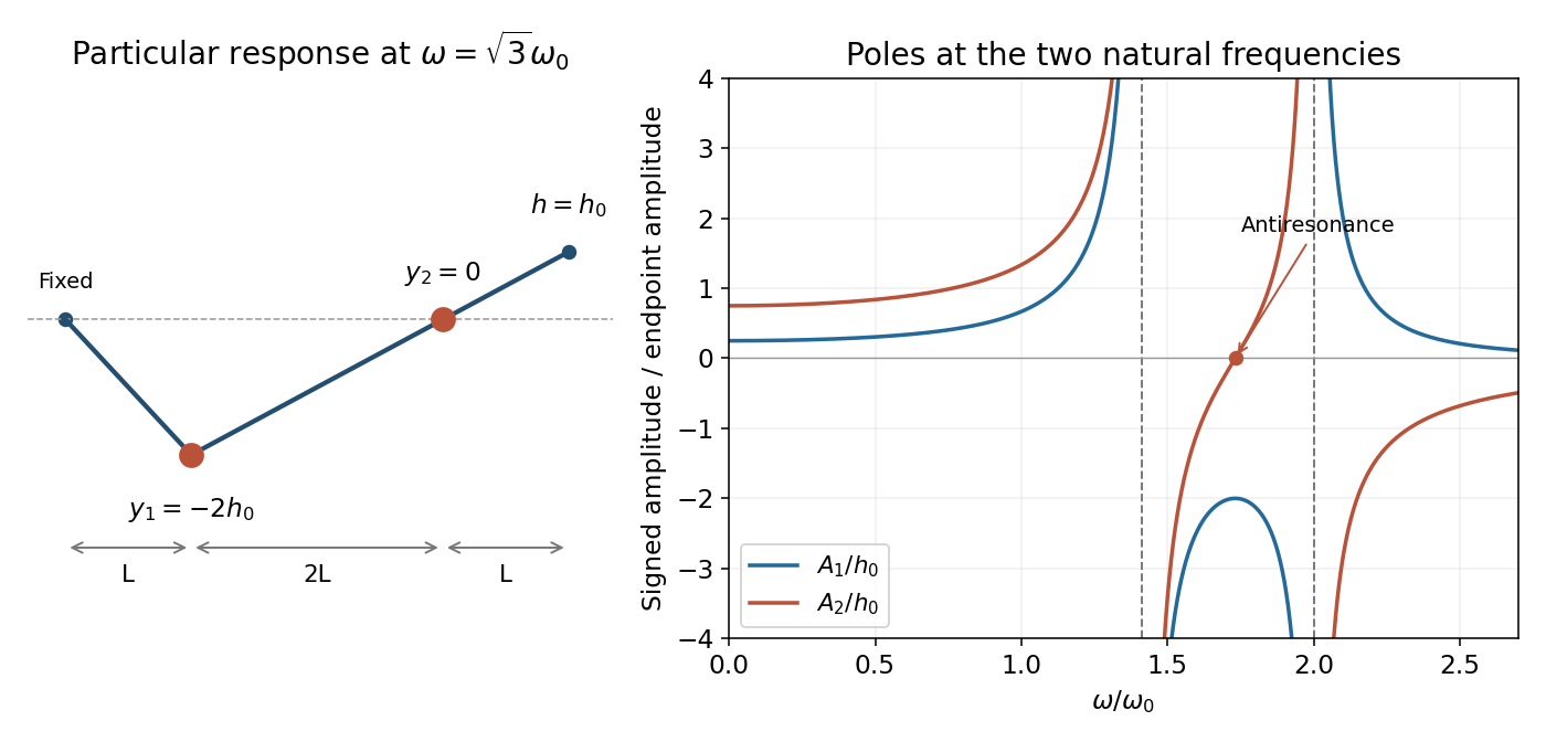
Periodic bead responses and the stationary second bead at antiresonance
. Details. As elsewhere in the undamped problem, this exact nodal motion presumes initial conditions selecting the periodic particular response. Additional free normal modes would move the second bead as well; they do not decay automatically.
Past exam of the mathematical methods II course of the University of Oxford 2015 resit 9 c Solution by Codex 0 2026-10-25
Codex 0 2026-10-25Away from the natural resonances, seek a periodic particular solution . Let . The amplitude equations areTheir determinant is , giving the signed displacement amplitudesA negative sign denotes a phase reversal relative to the prescribed cosine; physical amplitude magnitudes are . In the quasistatic limit,These are the values of a straight string interpolating between endpoint displacements and at bead positions and along a total length .
Because damping is explicitly absent, this periodic response is not a unique attracting late-time state. Arbitrary homogeneous oscillations at and persist unless the initial conditions eliminate them. At either natural resonance, the drive produces secular growth rather than a finite bounded periodic response. Thus “steady state” here refers to the selected particular solution away from the poles.
Past exam of the mathematical methods II course of the University of Oxford 2015 resit 9 b Solution by Codex 0 2026-10-25
Codex 0 2026-10-25The natural normal modes belong to the homogeneous system with both end displacements fixed at zero. Seek , soThe characteristic polynomial is . The eigenvectors and therefore giveThe symmetric mode leaves the middle segment horizontal, while the antisymmetric mode bends it strongly and has the higher restoring stiffness. Defining and diagonalizes the driven equations too:This shows that the boundary drive excites both natural modes; neither natural resonance is removed by a zero drive projection.
Past exam of the mathematical methods II course of the University of Oxford 2015 resit 9 a Solution by Codex 0 2026-10-25
Codex 0 2026-10-25The original diagram has three horizontal spans , and . In the small-slope approximation the massless string segments are straight and their transverse force components are tension times slope. The horizontal tension components cancel to first order.
For the first bead, the left segment contributes and the middle segment contributes . For the second bead, the middle contribution is and the driven right segment contributes . Newton's second law therefore givesWith and , the coupled equations of motion areThe factor two in the driving term follows from the right span having length , while the middle span has length . Treating all three spans as equal would change both the coupling and the normal mode frequencies.
Past exam of the mathematical methods II course of the University of Oxford 2015 resit 8 d Solution by Codex 0 2026-10-25
Codex 0 2026-10-25Take to be a simple closed, piecewise smooth curve oriented counterclockwise around its interior . Green's theorem applied to and givesThe orientation is essential: a clockwise unit circle gives , whereas twice its ordinary unsigned area is . For a nonsimple curve, the corresponding formula concerns signed area with winding multiplicity rather than one unsigned enclosed area.
Past exam of the mathematical methods II course of the University of Oxford 2015 resit 8 c Solution by Codex 0 2026-10-25
Codex 0 2026-10-25A one-form is an exact differential if a single-valued differentiable potential of a conservative vector field satisfies and on the domain. Then it equals , and its integral along a path is the endpoint difference of .
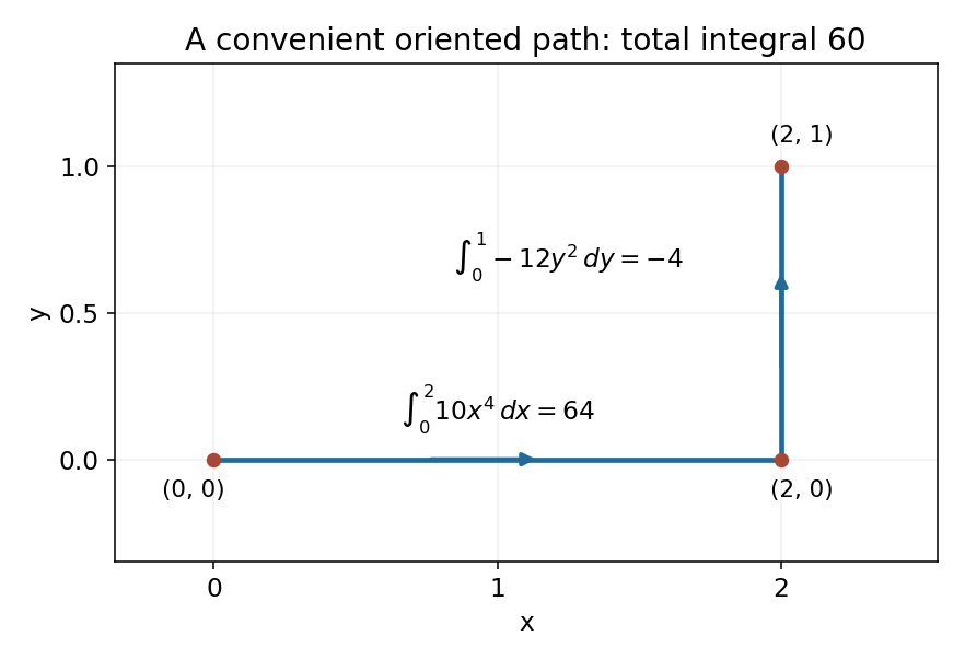
Integrate with respect to :Its derivative is . Matching the required second component forces , so the additive constant is arbitrary andThe fundamental theorem for line integrals now givesindependently of the convenient segmented path used before. Merely checking equality of mixed partial derivatives on an unspecified domain would not by itself construct this globally defined potential.
Past exam of the mathematical methods II course of the University of Oxford 2015 resit 8 b Solution by Codex 0 2026-10-25
Codex 0 2026-10-25Set and . Their mixed derivatives agree: . Both components are smooth on all of , a simply connected space, so the line integral is path independent.
Past exam of the mathematical methods II course of the University of Oxford 2015 resit 8 a Solution by Codex 0 2026-10-25
Codex 0 2026-10-25Embed the planar vector field as , independent of . Applying the Cartesian curl formula givesConsequently, for continuously differentiable components,This is the local closedness condition for the one-form . To infer global path independence from this condition alone, the domain also matters: it suffices that the planar domain is a simply connected space. The polynomial field in the next calculation is defined on the whole plane, so there is no missing-hole obstruction.
Past exam of the mathematical methods II course of the University of Oxford 2015 resit 6 c Solution by Codex 0 2026-10-25
Codex 0 2026-10-25The enclosed volume lies above and below . In cylindrical coordinates, its limits are , , , with volume element . The divergence theorem givesThus the volume is , and the outward flux is .
A direct check separates the boundary into its cap and base. On the base, . On the graph , the upward vector area element is , so the cap flux is , in agreement with the volume calculation.
Past exam of the mathematical methods II course of the University of Oxford 2015 resit 6 b Solution by Codex 0 2026-10-25
Codex 0 2026-10-25Read the given vector field as the three-dimensional field . Its divergence is the sum of the three matching-coordinate partial derivatives:The absence of a component does not make the three-dimensional flux vanish: the field still flows outward through surface normals with horizontal components.
Past exam of the mathematical methods II course of the University of Oxford 2015 resit 6 a Solution by Codex 0 2026-10-25
Codex 0 2026-10-25The divergence theorem states that, for a sufficiently smooth vector field on a volume with piecewise smooth closed boundary ,Here is the outward unit normal. The left-hand side is the total outward flux; the right-hand side adds the local divergence throughout the volume. The orientation and the requirement to include the complete closed boundary are essential.
Past exam of the mathematical methods II course of the University of Oxford 2015 resit 5 ii Solution by Codex 0 2026-10-25
Codex 0 2026-10-25Let and . Its partial derivatives areso both vanish at and . Evaluating the second derivatives at a point with givesTherefore the Hessian determinant is . Its two diagonal entries are negative at and positive at . HenceThese are also global extrema: for positive , the factor maximizes the positive value at , and differentiating fixes its positive maximum at . Oddness in supplies the corresponding global minimum.
Past exam of the mathematical methods II course of the University of Oxford 2015 resit 5 i Solution by Codex 0 2026-10-25
Codex 0 2026-10-25For a twice continuously differentiable function , first check the stationary-point condition . Write its Hessian matrix as , with , and . The second-derivative test uses : if and , the point is a strict local minimum; if and , it is a strict local maximum; if , it is a saddle point. If , the quadratic test is inconclusive and higher-order terms or a direct argument are needed.
For , the first derivatives vanish at the origin andThus . Directly, for nearby nonzero , while for nearby nonzero . The presence of both increasing and decreasing directions confirms the Hessian matrix classification.
Past exam of the mathematical methods II course of the University of Oxford 2015 resit 2 c Solution by Codex 0 2026-10-25
Codex 0 2026-10-25Let . The trigonometric identity changes the expression to . Since ,The negative sign is also forced geometrically: near its maximum, is negative while the numerator is nonnegative. Both numerator and denominator vanish quadratically, so one application of a first-derivative argument alone would not yet resolve the indeterminate form.
Past exam of the mathematical methods II course of the University of Oxford 2015 resit 2 b Solution by Codex 0 2026-10-25
Codex 0 2026-10-25Combine the two singular terms before taking the limit:For near zero, within the real domain , the Maclaurin series is . HenceThe two individual terms have divergent limits; their leading singularities cancel. Evaluating them separately as an “infinity minus infinity” subtraction would not justify the finite result.
Past exam of the mathematical methods II course of the University of Oxford 2015 resit 2 a Solution by Codex 0 2026-10-25
Codex 0 2026-10-25The Maclaurin series give and . Therefore , and cancellation of the common leading power givesThe argument applies from either side of zero: both leading terms involve the even power . The expression need not be defined at zero itself for its limit to exist.
Pinned article: Introduction to the OurBigBook Project
Welcome to the OurBigBook Project! Our goal is to create the perfect publishing platform for STEM subjects, and get university-level students to write the best free STEM tutorials ever.
Everyone is welcome to create an account and play with the site: ourbigbook.com/go/register. We belive that students themselves can write amazing tutorials, but teachers are welcome too. You can write about anything you want, it doesn't have to be STEM or even educational. Silly test content is very welcome and you won't be penalized in any way. Just keep it legal!
Intro to OurBigBook
. Source. We have two killer features:
- topics: topics group articles by different users with the same title, e.g. here is the topic for the "Fundamental Theorem of Calculus" ourbigbook.com/go/topic/fundamental-theorem-of-calculusArticles of different users are sorted by upvote within each article page. This feature is a bit like:
- a Wikipedia where each user can have their own version of each article
- a Q&A website like Stack Overflow, where multiple people can give their views on a given topic, and the best ones are sorted by upvote. Except you don't need to wait for someone to ask first, and any topic goes, no matter how narrow or broad
This feature makes it possible for readers to find better explanations of any topic created by other writers. And it allows writers to create an explanation in a place that readers might actually find it.
Figure 1. Screenshot of the "Derivative" topic page. View it live at: ourbigbook.com/go/topic/derivativeVideo 2. OurBigBook Web topics demo. Source. - local editing: you can store all your personal knowledge base content locally in a plaintext markup format that can be edited locally and published either:This way you can be sure that even if OurBigBook.com were to go down one day (which we have no plans to do as it is quite cheap to host!), your content will still be perfectly readable as a static site.
- to OurBigBook.com to get awesome multi-user features like topics and likes
- as HTML files to a static website, which you can host yourself for free on many external providers like GitHub Pages, and remain in full control

Figure 2. You can publish local OurBigBook lightweight markup files to either OurBigBook.com or as a static website.
Figure 3. Visual Studio Code extension installation.
Figure 5. . You can also edit articles on the Web editor without installing anything locally. Video 3. Edit locally and publish demo. Source. This shows editing OurBigBook Markup and publishing it using the Visual Studio Code extension. 
- Infinitely deep tables of contents:




All our software is open source and hosted at: github.com/ourbigbook/ourbigbook
Further documentation can be found at: docs.ourbigbook.com
Feel free to reach our to us for any help or suggestions: docs.ourbigbook.com/#contact