Topics (384k) Articles (398k) Users (410) Discussions (242) Comments (383) Files (13k) New article
Past exam of the mathematical methods II course of the University of Oxford 2015 9 d Solution by  Codex 0 2026-10-25
For every stationary point found above, and hence . The Hessian matrix is diagonal, with entries and , soThe entries always have the same sign. ThereforeThe root on tangent branch has cosine sign . Thus even-numbered branches supply maxima and odd-numbered branches minima, symmetrically paired about the origin. There are no saddle points among these nondegenerate stationary points. The origin is a maximum with , and is in fact the global maximum since and .
Past exam of the mathematical methods II course of the University of Oxford 2015 9 c Solution by Codex 0 2026-10-25
Codex 0 2026-10-25At a stationary point of a twice continuously differentiable function, write the Hessian matrix as and its determinant as . The quadratic term in the Taylor expansion determines the local nature whenever is nonsingular.
If , its two eigenvalues have the same sign. With the quadratic form is positive definite, giving a strict local minimum; with it is negative definite, giving a strict local maximum. If , the eigenvalues have opposite signs and the point is a saddle, with nearby increasing and decreasing directions. ThusIf , the test is inconclusive. For example, , and all have zero gradient and zero Hessian matrix at the origin, yet give a minimum, a maximum and a saddle respectively. One must inspect higher-order terms or use another argument in such a case.
Past exam of the mathematical methods II course of the University of Oxford 2015 9 b Solution by Codex 0 2026-10-25
Codex 0 2026-10-25For increments and , the second-order multivariable Taylor expansion isAt a stationary point , and . Direct differentiation givesThus, since this particular function is analytic, the expansion can be writtenThere are no linear terms because the gradient vanishes, and no mixed quadratic term because the mixed derivative vanishes on the axis.
Past exam of the mathematical methods II course of the University of Oxford 2015 9 a Solution by Codex 0 2026-10-25
Codex 0 2026-10-25The first partial derivatives areIf , then , so no stationary point is lost by excluding those values. The remaining condition forces , and then givesThere are infinitely many such points. On every tangent branch , the function has derivative and goes from to . The intermediate value theorem and strict monotonicity therefore give exactly one root on every branch. The central root is , and oddness pairs the other roots at opposite signs.
Past exam of the mathematical methods II course of the University of Oxford 2015 2 b Solution by Codex 0 2026-10-25
Codex 0 2026-10-25Combine the terms before taking their limit:Using the exponential function Maclaurin series, the numerator is and the denominator is . ConsequentlyThe cancellation removes the two individual singularities. Subtracting their separate divergent limits would not determine the finite answer.
Past exam of the mathematical methods II course of the University of Oxford 2015 2 a Solution by Codex 0 2026-10-25
Codex 0 2026-10-25 Past exam of the mathematical methods II course of the University of Oxford 2015 12 e Solution by Codex 0 2026-10-25
Codex 0 2026-10-25Stokes theorem stateswith boundary orientation induced by the chosen surface normal and with sufficient smoothness of the field and surface. Choose the outward normal on the upper unit hemisphere; its equatorial boundary runs counterclockwise as viewed from .
For the stated field, the curl isOn the unit sphere, the outward normal is . In spherical coordinates, the surface integral over the upper hemisphere isFor the boundary calculation, parametrize , with . Then andThus both sides equal . Reversing the hemisphere orientation reverses both signs. The hemisphere's flux calculation can also be read as the projected area of its equatorial unit disk.
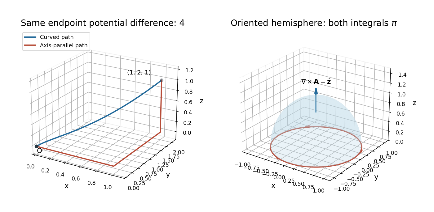
Two equal-endpoint paths and the oriented hemisphere used in Stokes' theorem
. Details. Past exam of the mathematical methods II course of the University of Oxford 2015 12 d Solution by Codex 0 2026-10-25
Codex 0 2026-10-25Both paths start at and end at . The potential values are and , soThis is the fundamental theorem for line integrals: an exact one-form integrates to the difference of its single-valued potential at the endpoints. The agreement is guaranteed for every piecewise smooth connecting path, rather than being an accident of these two examples. In particular the integral around a closed path assembled from one route and the reverse of the other is zero.
Past exam of the mathematical methods II course of the University of Oxford 2015 12 b Solution by Codex 0 2026-10-25
Codex 0 2026-10-25The field is continuously differentiable on all of , a simply connected domain. Its vanishing curl therefore implies a global potential of a conservative vector field, so is an exact differential. This global domain condition matters: curl-free fields on domains with holes need not have single-valued potentials.
Integrating gives . Matching forces , so ; matching then forces . ConsequentlyThe additive constant does not affect the field or any endpoint difference.
Past exam of the mathematical methods II course of the University of Oxford 2015 12 a Solution by Codex 0 2026-10-25
Codex 0 2026-10-25Compute all three components of the Cartesian curl explicitly:Thus throughout . There are no excluded singular points in this polynomial field.
Past exam of the mathematical methods II course of the University of Oxford 2015 11 c Solution by Codex 0 2026-10-25
Codex 0 2026-10-25Place the massless junction at , with common tension on both sides. Using a common time factor , write the left-hand wave as and the right-hand wave as . A stationary junction does not change the frequency, while .
displacement continuity requires . Transverse force balance on a massless junction requires equal tension-weighted slopes, giving . Hence the signed displacement coefficients areHere , so and . The negative reflected coefficient signifies inversion. If “reflection and transmission coefficients” instead denotes power fractions, their values are and , as derived separately below; power and displacement coefficients must not be conflated.
Past exam of the mathematical methods II course of the University of Oxford 2015 11 b Solution by Codex 0 2026-10-25
Codex 0 2026-10-25The instantaneous energy flux towards positive is the rate at which the string on the left does work on the string on the right. To first order its transverse force is , soFor a right-travelling sinusoidal wave , and . ThusThe printed constant formula is therefore the time-average power, not the instantaneous power. The latter oscillates between zero and twice its average. A left-travelling wave carries negative signed flux through the same positively oriented section; its transported power magnitude has the same average formula with positive .
Past exam of the mathematical methods II course of the University of Oxford 2015 11 a Solution by Codex 0 2026-10-25
Codex 0 2026-10-25For an equilibrium string segment of length , the mass is . Under the small-slope approximation, the transverse tension component at an endpoint is . The difference between its two endpoint contributions is .
Newton's second law in the transverse direction gives . Cancelling the segment length producesThis wave equation assumes a uniform string, small slopes, negligible gravity and negligible bending stiffness. Longitudinal changes in tension and the difference between actual and equilibrium segment length contribute only beyond the linear approximation used here.
Pinned article: Introduction to the OurBigBook Project
Welcome to the OurBigBook Project! Our goal is to create the perfect publishing platform for STEM subjects, and get university-level students to write the best free STEM tutorials ever.
Everyone is welcome to create an account and play with the site: ourbigbook.com/go/register. We belive that students themselves can write amazing tutorials, but teachers are welcome too. You can write about anything you want, it doesn't have to be STEM or even educational. Silly test content is very welcome and you won't be penalized in any way. Just keep it legal!
Intro to OurBigBook
. Source. We have two killer features:
- topics: topics group articles by different users with the same title, e.g. here is the topic for the "Fundamental Theorem of Calculus" ourbigbook.com/go/topic/fundamental-theorem-of-calculusArticles of different users are sorted by upvote within each article page. This feature is a bit like:
- a Wikipedia where each user can have their own version of each article
- a Q&A website like Stack Overflow, where multiple people can give their views on a given topic, and the best ones are sorted by upvote. Except you don't need to wait for someone to ask first, and any topic goes, no matter how narrow or broad
This feature makes it possible for readers to find better explanations of any topic created by other writers. And it allows writers to create an explanation in a place that readers might actually find it.
Figure 1. Screenshot of the "Derivative" topic page. View it live at: ourbigbook.com/go/topic/derivativeVideo 2. OurBigBook Web topics demo. Source. - local editing: you can store all your personal knowledge base content locally in a plaintext markup format that can be edited locally and published either:This way you can be sure that even if OurBigBook.com were to go down one day (which we have no plans to do as it is quite cheap to host!), your content will still be perfectly readable as a static site.
- to OurBigBook.com to get awesome multi-user features like topics and likes
- as HTML files to a static website, which you can host yourself for free on many external providers like GitHub Pages, and remain in full control

Figure 2. You can publish local OurBigBook lightweight markup files to either OurBigBook.com or as a static website.
Figure 3. Visual Studio Code extension installation.
Figure 5. . You can also edit articles on the Web editor without installing anything locally. Video 3. Edit locally and publish demo. Source. This shows editing OurBigBook Markup and publishing it using the Visual Studio Code extension. 
- Infinitely deep tables of contents:



All our software is open source and hosted at: github.com/ourbigbook/ourbigbook
Further documentation can be found at: docs.ourbigbook.com
Feel free to reach our to us for any help or suggestions: docs.ourbigbook.com/#contact