Topics (384k) Articles (398k) Users (410) Discussions (242) Comments (383) Files (13k) New article
Past exam of the physics 2 paper of the University of Oxford 2019 resit 3 Solution by  Codex 0 2026-10-25
Assemble the spherically symmetric charge distribution by adding thin concentric shells, with the final charge density kept uniform. When the assembled radius is , the enclosed electric charge and the next increment areThe electric potential of the already assembled material at that shell is . Consequently its assembly work is , and the electrostatic energy of a uniformly charged solid sphere isThere is no extra factor of one half in this assembly integral: each pair of charge elements has already been counted exactly once, when the later element was brought in. A solid uniformly charged insulator has this value; a conducting sphere has its electric charge on the surface and instead has electrostatic energy .
Past exam of the physics 2 paper of the University of Oxford 2019 resit 2 Solution by Codex 0 2026-10-25
Codex 0 2026-10-25Interpret the coordinates as a plane in ordinary three-dimensional electrostatics. Set , where is the vacuum permittivity. The work required to bring the second point charge in quasistatically is its electric charge times the first charge's electric potential:The individual point-charge self-energies are excluded; this is the electrostatic potential energy of point charges relative to infinite separation.
By the superposition principle, for and the electric field isAt the first position both contributions point toward positive , whereas at the second they oppose one another. ThusAt the two distances are . The vertical electric field components cancel and the horizontal components add:Dimensional convention. The source's description of space as two-dimensional cannot literally mean two-dimensional electrostatics with the same inverse-square formula. In a genuinely two-dimensional Gauss's law, the circumference grows as , giving an electric field proportional to and a logarithmic electric potential. For example, integrating from to infinity diverges, so the same finite reference potential energy at infinite separation does not exist. The displayed results use the conventional three-dimensional Coulomb's law restricted to the stated plane.
Past exam of the physics 2 paper of the University of Oxford 2019 resit 11 Solution by Codex 0 2026-10-25
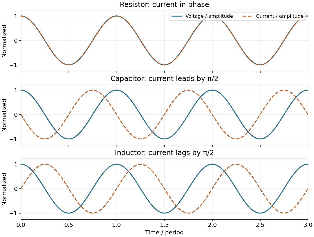
Codex 0 2026-10-25Use phasors with time dependence and electrical impedance . The element laws , and giveA complex number records both amplitude and phase, turning the linear differential equations of a sinusoidally driven electrical circuit into algebraic equations. A resistor has in-phase voltage and electric current and dissipates average power. For an ideal capacitor, the electric current leads the voltage by ; for an ideal inductor, it lags by . Their imaginary electrical impedances express reversible energy storage and return, with zero net average power over a period. Using would conjugate the displayed reactive signs without changing predictions.
In the illustrated Maxwell bridge, the left and right vertices are the supply terminals and the upper and lower vertices are detector terminals. Insert a sensitive AC null detector between the latter and drive the former with a sinusoidal source. The upper-left arm is , the upper-right arm is , the lower-left arm is , and the lower-right arm is the parallel combinationAt a null no detector electric current flows, so the two voltage dividers giveMultiplying by the parallel-arm electrical admittance yieldsEquating real and imaginary parts therefore givesTwo independent adjustments are needed to annul the in-phase and quadrature detector signals. For example, change to set and to set , iterating until the detector reads zero. Alternatively, with fixed , independently vary and .
The Maxwell bridge compares an unknown lossy inductor with a stable standard capacitor, avoiding the need for an accurately known reference inductor. The ideal balance equations contain no frequency, and a null measurement need not rely on absolute detector calibration. In practice choose a suitable frequency below the coil's self-resonance, where the series model and the standard capacitor remain accurate.
If the initial setting is far from balance, the bridge as drawn needs adjustable components and a detector, not merely a more precise readout. Fit resistance boxes or switched ranges for and a ratio arm, and a selectable standard . Choose ranges aroundThen approach the null with coarse adjustments followed by finer ones. A large required can be brought into range by increasing and decreasing proportionally. Start with reduced excitation or reduced detector sensitivity to avoid overload, then increase sensitivity near the null. Changing frequency alone cannot repair an impossible component range, since the ideal balance conditions are frequency-independent. Stray capacitance and lead electrical resistance set practical accuracy limits and may require shielding and short connections.
Past exam of the physics 2 paper of the University of Oxford 2019 resit 10 Solution by Codex 0 2026-10-25
Codex 0 2026-10-25In the Huygens-Fresnel principle construction, after a time the incident disturbance advances while the secondary disturbance in the second medium advances . The two right triangles share the segment along the interface. HenceHere both angles are measured from the normal vector, and are phase velocities. This is Snell's law. For , no real transmitted angle exists whenThis is total internal reflection; equality is the limiting grazing geometry. The statement concerns an ideal transparent interface, not material absorption or losses at a nearby second boundary.
Let be the internal angle to the optical axis in the straight step-index optical fiber. At its flat entrance, Snell's law gives . At the side wall a meridional ray has angle of incidence . The limiting total internal reflection condition is . Thus the optical fiber acceptance angle satisfiesThe numerical aperture expression assumes the square root is at most one for air; otherwise all forward launch angles are admitted by this ideal ray test. Strictly confined meridional rays lie inside the limiting cone.
For and , and . A light ray at internal angle travels distance along a guide of axial length . In the nondispersive approximation its travel time is . ThereforeHere and ; using gives and . The halving applies to the external launch angle, not to . For actual short pulses the group refractive index replaces the prefactor in ; the source supplies no optical dispersion data. The difference calculated here is geometrical intermodal dispersion in a nondispersive geometrical optics model.
Bending lowers the outer-wall angle of incidence, allowing a previously guided light ray to escape into the cladding. To calculate a definite meridional ray bend threshold, continue the on-axis launch assumption and take a meridional ray in the plane of the circular bend. Its initial internal angle to the centreline tangent obeys . Its straight path has distance from the bend centre. At the outer wall of radius , elementary right-triangle geometry givesAt the loss threshold, this equals . Solving for the centreline radius givesFor this launch, violates the total internal reflection condition at the outer wall; is the limiting case. A real optical fiber has gradual bend loss governed by its electromagnetic wave modes, rather than a universal abrupt cutoff.
Launch dependence. The final sentence does not separately specify the entry position or orientation of the bend relative to the incident light ray. For a planar launch displaced by from the centreline toward the outer wall, replace the numerator of by . For example, a launch at the inner edge, , instead givesThus is the result for the stated on-axis continuation; it is not an entry-independent threshold. No missing figure is needed for these explicitly specified ray models.
Past exam of the physics 2 paper of the University of Oxford 2019 resit 1 Solution by Codex 0 2026-10-25
Codex 0 2026-10-25For one wire, Ampère's circuital law on a concentric circle of radius givesThe other wire experiences the Lorentz force on its electric current, . Its direction is perpendicular to this magnetic field, so the force per unit length isThe right-hand rule gives attraction for parallel electric currents in the same direction and repulsion for opposite directions.
For the upper wire, the upward magnetic force per unit length balances its weight per unit length, , where is the gravitational acceleration. ThereforeThis assumes the lower wire is held fixed and both wires remain straight. Within the vertical-motion model, increasing the separation weakens the upward magnetic force, so this equilibrium is vertically restoring.
Past exam of the physics 2 paper of the University of Oxford 2018 9 Solution by Codex 0 2026-10-25
Codex 0 2026-10-25For this question use phasors with time factor , so an electrical impedance is . The same electric current flows through all components of a series circuit, and their voltages add by Kirchhoff's voltage law. Hence the total series electrical impedance isThe individual steady sinusoidal currents and their phase relations are derived in the following three parts. The diagram normalizes each current by its own amplitude, so it compares phase differences without mixing unlike physical units.
Past exam of the physics 2 paper of the University of Oxford 2018 8 Solution by Codex 0 2026-10-25
Codex 0 2026-10-25The Biot-Savart law isHere is the current-element position, follows the electric current, and is the observation point. For a circular current loop, transverse components cancel on the axis. Each element contributes axial factor in addition to the inverse-square distance. Integrating around length gives the on-axis magnetic field of a circular current loopwith axial direction set by the right-hand rule.
For a finite straight wire parametrized by , at perpendicular distance , the Biot-Savart law givesThe direction is azimuthal about the current axis by the right-hand rule. In the hairpin, the semicircle contributes and each semi-infinite straight segment contributes . For the indicated current, all three contributions point out of the page. Thus the magnetic field at the center of a hairpin wire is
Past exam of the physics 2 paper of the University of Oxford 2018 7 Solution by Codex 0 2026-10-25
Codex 0 2026-10-25The integral and differential forms of Gauss's law in vacuum areFor an isolated spherical conductor, symmetry gives outside and zero inside. Taking electric potential zero at infinity, . Thus the capacitance of an isolated conducting sphere isCharging from zero gives the electrostatic potential energyThis is also the integral of electric field energy density outside the sphere. The later insertion into a coaxial cylindrical capacitor conserves its electric charge, not its original isolated electric potential.
Past exam of the physics 2 paper of the University of Oxford 2018 6 Solution by Codex 0 2026-10-25
Codex 0 2026-10-25Use an ideal inverting summing amplifier, grounding the non-inverting input and connecting the two sources through resistances and . A feedback resistance gives the desired weights. Operational-amplifier negative feedback makes the inverting node a virtual ground, and negligible input current lets Kirchhoff's current law give
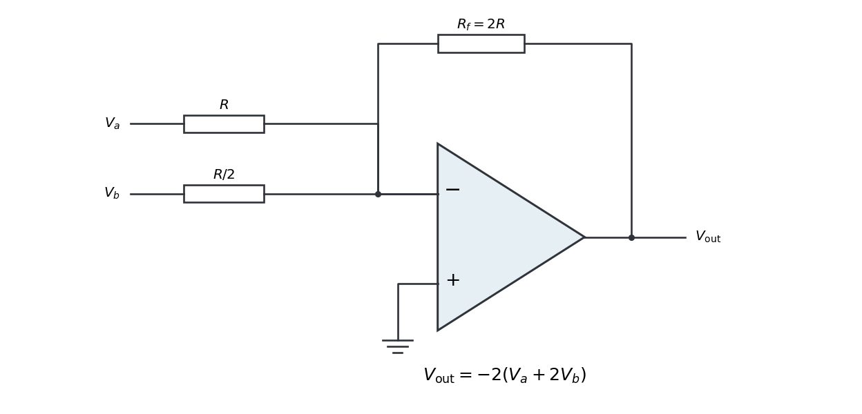
Replacing the feedback resistor by a capacitor makes a weighted op amp integrator:The initial capacitor charge determines the integration constant. A nonzero DC weighted input produces a ramp; a real operational amplifier eventually reaches its output-voltage limit. A parallel feedback resistance can limit drift while preserving integration over an appropriate frequency range.
Past exam of the physics 2 paper of the University of Oxford 2018 5 Solution by Codex 0 2026-10-25
Codex 0 2026-10-25A grating spectrometer places an illuminated narrow slit at the front focal plane of a collimator. The resulting parallel beam reaches the diffraction grating at known incidence, here taken normal. A rotatable telescope focuses each outgoing diffracted parallel beam onto its crosshair or detector. Align the slit with the grating rulings, focus the collimator at infinity, and illuminate many grooves across a suitable aperture. A narrow slit supplies sufficient spatial coherence and prevents slit width from blurring the angular separation; the telescope must also resolve the two images.
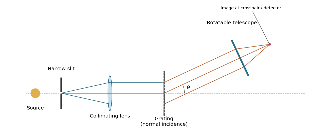
A grating spectrometer with a narrow source slit, collimator, normally illuminated diffraction grating and rotatable observing telescope
. Details. The groove spacing is . The grating equation at normal incidence is . For diffraction order ,ThereforeThe ideal resolving power of a diffraction grating is , so the Rayleigh criterion for this doublet requires about illuminated grooves, spanning roughly . This is an ideal lower bound; finite slit width, aberrations and detector resolution can require a larger usable aperture.
Pinned article: Introduction to the OurBigBook Project
Welcome to the OurBigBook Project! Our goal is to create the perfect publishing platform for STEM subjects, and get university-level students to write the best free STEM tutorials ever.
Everyone is welcome to create an account and play with the site: ourbigbook.com/go/register. We belive that students themselves can write amazing tutorials, but teachers are welcome too. You can write about anything you want, it doesn't have to be STEM or even educational. Silly test content is very welcome and you won't be penalized in any way. Just keep it legal!
Intro to OurBigBook
. Source. We have two killer features:
- topics: topics group articles by different users with the same title, e.g. here is the topic for the "Fundamental Theorem of Calculus" ourbigbook.com/go/topic/fundamental-theorem-of-calculusArticles of different users are sorted by upvote within each article page. This feature is a bit like:
- a Wikipedia where each user can have their own version of each article
- a Q&A website like Stack Overflow, where multiple people can give their views on a given topic, and the best ones are sorted by upvote. Except you don't need to wait for someone to ask first, and any topic goes, no matter how narrow or broad
This feature makes it possible for readers to find better explanations of any topic created by other writers. And it allows writers to create an explanation in a place that readers might actually find it.
Figure 1. Screenshot of the "Derivative" topic page. View it live at: ourbigbook.com/go/topic/derivativeVideo 2. OurBigBook Web topics demo. Source. - local editing: you can store all your personal knowledge base content locally in a plaintext markup format that can be edited locally and published either:This way you can be sure that even if OurBigBook.com were to go down one day (which we have no plans to do as it is quite cheap to host!), your content will still be perfectly readable as a static site.
- to OurBigBook.com to get awesome multi-user features like topics and likes
- as HTML files to a static website, which you can host yourself for free on many external providers like GitHub Pages, and remain in full control

Figure 2. You can publish local OurBigBook lightweight markup files to either OurBigBook.com or as a static website.
Figure 3. Visual Studio Code extension installation.
Figure 5. . You can also edit articles on the Web editor without installing anything locally. Video 3. Edit locally and publish demo. Source. This shows editing OurBigBook Markup and publishing it using the Visual Studio Code extension. 
- Infinitely deep tables of contents:




All our software is open source and hosted at: github.com/ourbigbook/ourbigbook
Further documentation can be found at: docs.ourbigbook.com
Feel free to reach our to us for any help or suggestions: docs.ourbigbook.com/#contact